python打卡训练营打卡记录day22

复习日
仔细回顾一下之前21天的内容，没跟上进度的同学补一下进度。

作业：

自行学习参考如何使用kaggle平台，写下使用注意点，并对下述比赛提交代码

kaggle泰坦尼克号人员生还预测

导入数据

# 导入所需库
import pandas as pd
import numpy as np
import matplotlib.pyplot as plt
import seaborn as sns
import warnings
from sklearn.model_selection import train_test_split, GridSearchCV
from sklearn.preprocessing import StandardScaler
from sklearn.metrics import accuracy_score, classification_report, confusion_matrix
from sklearn.impute import SimpleImputer
from lightgbm import LGBMClassifier
import shap

# 忽略警告
warnings.filterwarnings("ignore")

# 设置中文字体
plt.rcParams['font.sans-serif'] = ['SimHei']
plt.rcParams['axes.unicode_minus'] = False

# 加载数据
train_data = pd.read_csv('train.csv')
test_data = pd.read_csv('test.csv')

数据预处理

# 删除无关列
drop_columns = ['PassengerId', 'Name', 'Ticket', 'Cabin']
train_data = train_data.drop(drop_columns, axis=1)
test_data = test_data.drop(drop_columns, axis=1)

# 性别0-1编码
train_data['Sex'] = train_data['Sex'].map({'female': 0, 'male': 1})
test_data['Sex'] = test_data['Sex'].map({'female': 0, 'male': 1})

# Embarked独热编码
train_data = pd.get_dummies(train_data, columns=['Embarked'], drop_first=True)
test_data = pd.get_dummies(test_data, columns=['Embarked'], drop_first=True)

# 填充缺失值（年龄和票价用中位数）
imputer_age = SimpleImputer(strategy='median')
train_data['Age'] = imputer_age.fit_transform(train_data[['Age']])
test_data['Age'] = imputer_age.transform(test_data[['Age']])

imputer_fare = SimpleImputer(strategy='median')
train_data['Fare'] = imputer_fare.fit_transform(train_data[['Fare']])
test_data['Fare'] = imputer_fare.transform(test_data[['Fare']])

特征工程

# 添加家庭规模和独自旅行特征
train_data['FamilySize'] = train_data['SibSp'] + train_data['Parch'] + 1  # 家庭规模（包括自己）
train_data['IsAlone'] = (train_data['FamilySize'] == 1).astype(int)  # 1表示独自旅行

test_data['FamilySize'] = test_data['SibSp'] + test_data['Parch'] + 1
test_data['IsAlone'] = (test_data['FamilySize'] == 1).astype(int)

调参与模型训练

X_train = train_data.drop('Survived', axis=1)
y_train = train_data['Survived']
X_test = test_data  # 测试集暂不使用，如需预测可后续添加

# 划分训练集和验证集（8:2）
X_train_split, X_val, y_train_split, y_val = train_test_split(
    X_train, y_train, test_size=0.2, random_state=42

# 定义参数网格
param_grid = {
    'n_estimators': [50, 100, 200],  
    'learning_rate': [0.05, 0.1, 0.2],  # 平衡速度与精度的常用值
    'max_depth': [5, 10],  
    'min_child_samples': [10, 20],  
    'subsample': [0.8, 1.0],  # 行抽样常用值
    'colsample_bytree': [0.8, 1.0]  # 列抽样常用值
}

# 初始化模型和网格搜索
model = LGBMClassifier(random_state=42, verbose=-1)
grid_search = GridSearchCV(
    estimator=model,
    param_grid=param_grid,
    cv=3,  # 3折交叉验证（比5折快40%）
    n_jobs=-1,
    scoring='f1_macro',
    verbose=1
)

# 执行网格搜索
grid_search.fit(X_train_split, y_train_split)

# 获取最优模型和参数
best_lgbm = grid_search.best_estimator_
print(f"最优参数：{grid_search.best_params_}")
print(f"最佳交叉验证F1值：{grid_search.best_score_:.4f}")

Fitting 3 folds for each of 144 candidates, totalling 432 fits
最优参数：{'colsample_bytree': 1.0, 'learning_rate': 0.1, 'max_depth': 10, 'min_child_samples': 20, 'n_estimators': 50, 'subsample': 0.8}
最佳交叉验证F1值：0.8099

模型评估

y_pred = best_lgbm.predict(X_val)

print("\n调优后LightGBM模型评估结果：")
print(f"准确率：{accuracy_score(y_val, y_pred):.4f}")
print("分类报告：")
print(classification_report(y_val, y_pred))
print("混淆矩阵：")
print(confusion_matrix(y_val, y_pred))

调优后LightGBM模型评估结果：
准确率：0.8324
分类报告：
              precision    recall  f1-score   support

           0       0.85      0.87      0.86       105
           1       0.81      0.78      0.79        74

    accuracy                           0.83       179
   macro avg       0.83      0.83      0.83       179
weighted avg       0.83      0.83      0.83       179

混淆矩阵：
[[91 14]
 [16 58]]

shap可视化

# 初始化SHAP解释器
explainer = shap.TreeExplainer(best_lgbm)
shap_values = explainer.shap_values(X_val)  # 二分类返回长度为2的列表，shap_values[1]对应类别1（生存）

# 提取类别1的SHAP值（形状：(n_samples, n_features)）
shap_values_class1 = shap_values[1]

# 1. 特征重要性汇总（柱状图）
plt.figure(figsize=(10, 6))  
shap.summary_plot(
    shap_values_class1, 
    X_val, 
    feature_names=X_train.columns, 
    plot_type="bar",
    show=False  
)
plt.title("SHAP特征重要性排名", fontsize=14)  
plt.tight_layout()  # 自动调整子图参数，避免重叠
plt.savefig("shap_feature_importance.png", dpi=300, bbox_inches='tight')  
plt.show()

# 2. 特征影响汇总（蜂群图）
plt.figure(figsize=(12, 8))  # 增大画布尺寸，适应更多元素
shap.summary_plot(
    shap_values_class1, 
    X_val, 
    feature_names=X_train.columns,
    show=False
)
plt.title("SHAP特征影响方向与强度", fontsize=14)
plt.tight_layout() 
plt.savefig("shap_summary_plot.png", dpi=300, bbox_inches='tight')
plt.show()

# 3. 单个特征依赖图（前6个特征）
plt.figure(figsize=(16, 12))  

for i, feature in enumerate(X_train.columns[:6]): 
    plt.subplot(2, 3, i + 1)  
    
    shap.dependence_plot(
        feature, 
        shap_values_class1, 
        X_val, 
        feature_names=X_train.columns, 
        show=False,  
        ax=plt.gca()  
    )
    
    plt.title(f"{feature} 对生存概率的影响", fontsize=12)  # 添加子图标题
    plt.xlabel(feature)  # 显式设置x轴标签

plt.tight_layout(pad=4)  # 增加子图间距，防止标题重叠
plt.savefig("shap_dependence_plots.png", dpi=300, bbox_inches='tight')
plt.show()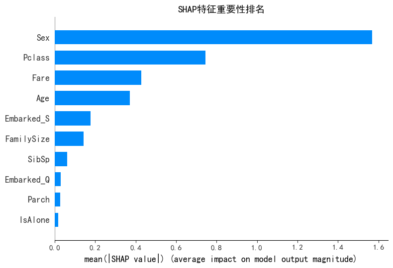

shap图分析

1. SHAP 特征重要性排名（柱状图）

• 横轴 ：mean(|SHAP value|)，表示特征对模型输出影响的平均绝对值，值越大说明特征越重要。
• 关键结论 ：
  • Sex：重要性最高，说明性别对生存概率影响最大。
  • Pclass：次之，客舱等级影响显著。
  • Fare、Age：也有较高影响，票价和年龄对模型决策有重要作用。
  • 其他特征（如 FamilySize、SibSp 等）影响较小。

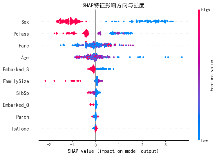
2. SHAP 特征影响方向与强度（蜂群图）

• 横轴：SHAP 值，正表示促进生存，负表示抑制生存。
• 点颜色：红色代表特征值高，蓝色代表特征值低。
• 关键结论 ：
  • Sex：红色点（特征值高）多在正 SHAP 值区域，说明该特征值高（如女性）时，显著促进生存；蓝色点（特征值低）在负区域，抑制生存。
  • Pclass：部分红色点在负 SHAP 值区域，表明客舱等级高（特征值高）可能抑制生存；蓝色点分布较分散，需结合具体值分析。
  • Fare：高值（红色）点多在正 SHAP 值区域，说明票价高促进生存。
  • Age：特征值与 SHAP 值无明显单调关系，但整体分布显示其对生存有复杂影响。

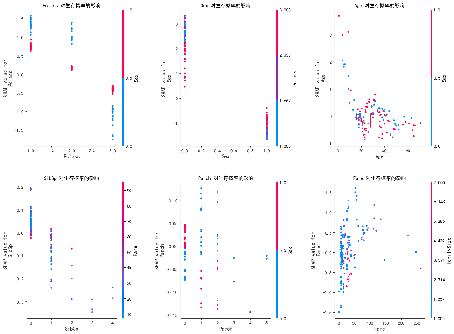
3. 单个特征依赖图（前 6 个特征）

• 横轴 ：特征值；纵轴 ：SHAP 值；点颜色：通常表示特征值高低（红色高，蓝色低）。
• 关键结论 ：
  • Pclass：低 Pclass 值（如 1 级舱位）对应正 SHAP 值，促进生存；高值（如 3 级）可能抑制生存。
  • Sex：特征值高（如女性）对应高正 SHAP 值，强烈促进生存。
  • Age：年轻乘客（低年龄值）SHAP 值多为正，促进生存；年长者 SHAP 值分散，影响复杂。
  • Fare：票价越高，SHAP 值越正，对生存促进作用越明显。
  • SibSp、Parch：值较低时，SHAP 值多为负，可能抑制生存；值较高时影响不明显。

综合总结

• 核心影响特征 ：Sex（性别）是决定生存概率的最关键因素，女性更易生存；Fare（票价）高、Age（年龄）小也显著促进生存。
• 客舱等级矛盾 ：Pclass 高（舱位等级低，如 3 级舱）反而可能抑制生存，与常识中 "高舱位更易生存" 看似矛盾，需结合数据具体分布进一步验证（如高舱位是否有更多特殊情况）。
• 家庭关系影响弱 ：SibSp（兄弟姐妹 / 配偶数）、Parch（父母 / 子女数）对生存影响较小，仅在特定值时表现出一定规律。

@浙大疏锦行