手搓传染病模型（SEIARW）

在传染病传播的研究中，水传播途径是一个重要的考量因素。SEAIRW 模型（易感者 S - 暴露者 E - 感染者 I - 无症状感染者 A - 康复者 R - 水中病原体 W）综合考虑了人与人接触传播以及水传播的双重机制，为分析此类传染病提供了全面的框架。图中的微分方程组清晰地定义了各变量的动态变化：

\(\begin{cases} \frac{dS}{dt} = -\beta S (I + kA) - \beta_w S W \\ \frac{dE}{dt} = \beta S (I + kA) + \beta_w S W - p\omega' E - (1 - p)\omega E \\ \frac{dI}{dt} = (1 - p)\omega E - \gamma I \\ \frac{dA}{dt} = p\omega' E - \gamma' A \\ \frac{dR}{dt} = \gamma I + \gamma' A \\ \frac{dW}{dt} = \mu I + \mu' A - \epsilon W \end{cases}\)

一、模型方程深度解析

易感者 S：\(\frac{dS}{dt} = -\beta S (I + kA) - \beta_w S W\)，表示易感者因接触感染者 I、无症状感染者 A（传播概率 k）以及水中病原体 W（传播系数 \(\beta_w\)）而减少。
暴露者 E：\(\frac{dE}{dt} = \beta S (I + kA) + \beta_w S W - p\omega' E - (1 - p)\omega E\)，包含感染输入（来自 S 的感染）、向无症状感染者（\(p\omega' E\)）和感染者（\((1 - p)\omega E\)）的转化。
感染者 I：\(\frac{dI}{dt} = (1 - p)\omega E - \gamma I\)，由暴露者转化而来（\((1 - p)\omega E\)），并以速率 \(\gamma\) 康复。
无症状感染者 A：\(\frac{dA}{dt} = p\omega' E - \gamma' A\)，由暴露者转化（\(p\omega' E\)），并以速率 \(\gamma'\) 康复。
康复者 R：\(\frac{dR}{dt} = \gamma I + \gamma' A\)，汇总感染者和无症状感染者的康复贡献。
水中病原体 W：\(\frac{dW}{dt} = \mu I + \mu' A - \epsilon W\)，包含感染者和无症状感染者向水中释放病原体（\(\mu I + \mu' A\)），以及病原体的自然去除（\(\epsilon W\)）。

二、MATLAB 代码实现细节

1. 参数与初始条件设置

Matlab 复制代码

md.b = 0.8;      % 易感者与感染者接触率
md.bW = 0.5;     % 易感者与水中病原体接触率
md.kappa = 0.05; % 无症状感染者向易感者传播的概率
md.p = 0.3;      % 成为无症状感染者的概率
md.omega = 1;    % 暴露者转为感染者的速率
md.omegap = 1;   % 暴露者转为无症状感染者的速率
md.gamma = 1/3;  % 感染者康复率
md.gammap = 0.03846; % 无症状感染者康复率
md.c = 0.48;     % 无症状感染者向水中释放病原体的速率
md.epsilon = 0.1; % 水中病原体去除速率
t = 1:1:100; % 模拟100天

% 初始比例
s0 = 798/800;  
i0 = 2/800;    
e0 = i0 / ((1-md.p) * md.omega); 
a0 = 0;        
r0 = 0;        
w0 = 0;        
N0 = 800;      
X0 = [s0, e0, i0, a0, r0, w0];

详细设定传播、转化、康复等速率参数，以及初始时刻各仓室的比例和水中病原体浓度。

2. 干预措施与模拟循环

Matlab 复制代码

itimes = 4; % 增加感染者的时间点
iamounts = 6; % 增加的感染者数量
stimes = 5; % 增加易感者的时间点
samounts = 600; % 增加的易感者数量

for idx = 1:length(t)  
    currenttime = t(idx);  
    if currenttime == itimes  
        X0(3) = (X0(3)*N0 + iamounts)/N0; % 增加感染者比例
        X0(1) = (X0(1)*N0 - iamounts)/N0; % 减少易感者比例
    end  
    if currenttime == stimes 
        N0 = N0 + samounts; % 更新总人口
        X0=X0.*((N0 - samounts)/N0); % 调整各仓室比例
        X0(1) = X0(1) + samounts/N0; % 增加易感者比例
    end  
    dXdt = SEAIRW_model(currenttime,X0, md);
    X0 = X0 + dXdt';  
    % 保存结果...
end

在特定时间点（第 4 天和第 5 天）实施干预，模拟现实中的疫情变化，如突发感染事件和人口流动。

3. 模型函数定义

Matlab 复制代码

function dXdt = SEAIRW_model(t, X, md)  
    s = X(1); e = X(2); i = X(3); a = X(4); r = X(5); w = X(6);  
    dsdt = -md.b * s * (i + md.kappa * a) - md.bW * s * w;  
    dedt = -dsdt - (md.p * md.omegap + (1-md.p) * md.omega) * e;  
    didt = (1-md.p) * md.omega * e - md.gamma * i;  
    dadt = md.p * md.omegap * e - md.gammap * a;  
    drdt = md.gamma * i + md.gammap * a;  
    dwdt = (i + a * md.c) * md.epsilon - md.epsilon * w;  
    dXdt = [dsdt; dedt; didt; dadt; drdt; dwdt];  
end

严格按照模型方程计算各变量的导数，确保模拟的准确性。

三、结果可视化与分析

通过绘图展示各变量随时间的变化：

Matlab 复制代码

figure; 
plot(S, 'k-', 'LineWidth', 1.5); hold on;
plot(E, 'g-', 'LineWidth', 1.5); 
plot(I, 'r-', 'LineWidth', 1.5); 
plot(A, 'm-', 'LineWidth', 1.5); 
plot(R, 'c-', 'LineWidth', 1.5); 
plot(W, 'b-', 'LineWidth', 1.5); 
legend('S', 'E', 'I', 'A', 'R', 'W','Location','east');
xlabel('Time(Day)');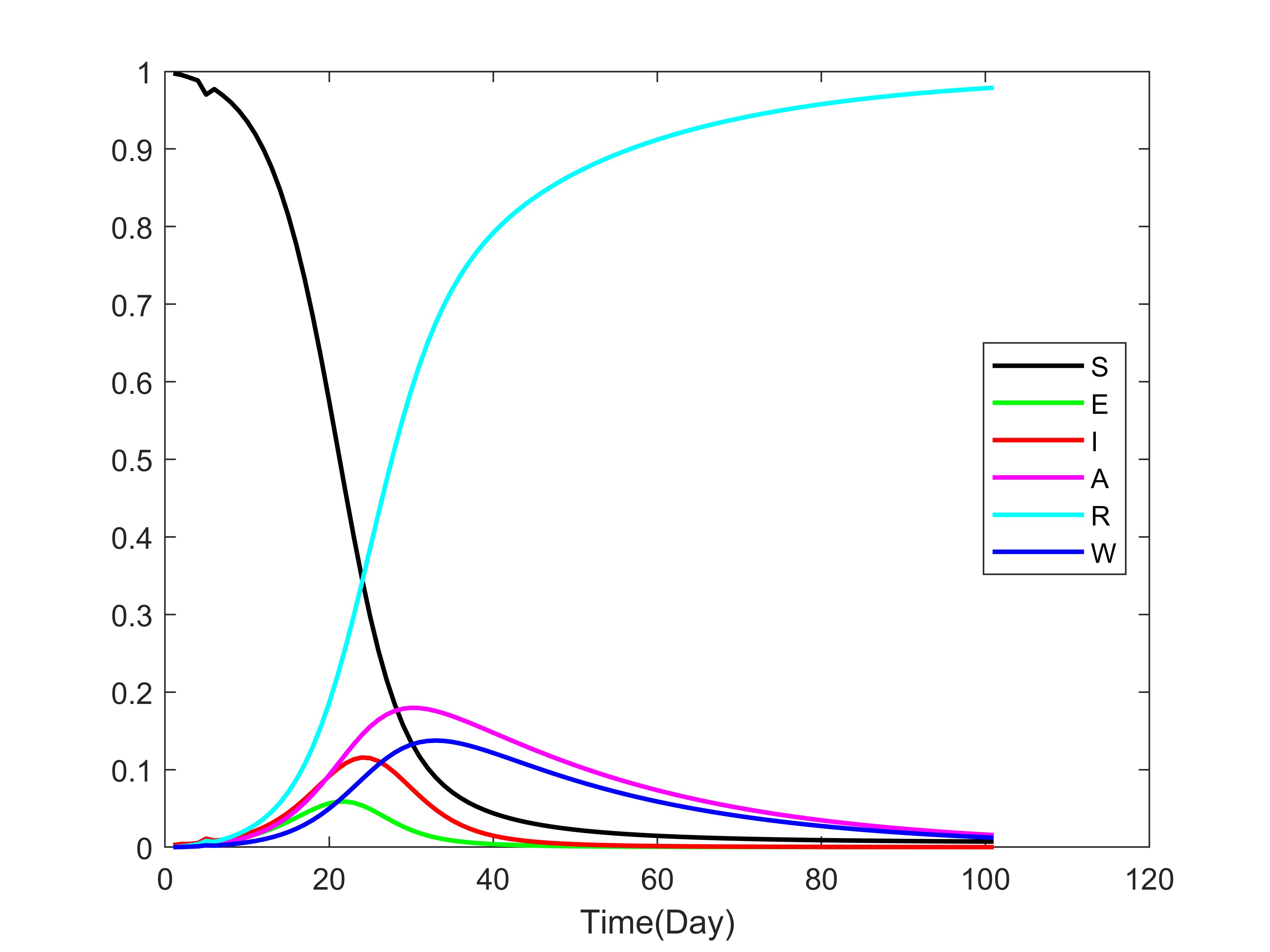

易感者 S 因感染逐渐减少，暴露者 E 先升后降，感染者 I 和无症状感染者 A 呈现动态变化，康复者 R 持续增加，水中病原体 W 随释放和去除机制波动。

四、模型应用与价值

SEAIRW 模型综合了接触传播和水传播途径，适用于霍乱、伤寒等水传播疾病的研究。通过 MATLAB 代码实现，能够模拟不同干预措施下的疫情发展，为公共卫生决策提供科学依据，如优化水源管理、制定隔离政策等。模型的灵活性和可扩展性使其成为分析复杂传染病传播的有力工具。

通过深入理解 SEAIRW 模型及其 MATLAB 实现，我们能够更有效地应对水传播传染病的挑战，为保障公众健康提供坚实的支持。快来尝试调整参数，探索不同场景下的疫情动态吧！ 💻🦠

完整代码（省流版）

Matlab 复制代码

close all; clear; clc;
% # Initial parameter settings
md.b = 0.8;      % Contact rate between susceptible and infected individuals
md.bW = 0.5;     % Contact rate between susceptible and infected in water
md.kappa = 0.05; % The probability of transmission from asymptomatic to susceptible
md.p = 0.3;      % The probability of being asymptomatic
md.omega = 1;    % Transition rate from exposed to infectious
md.omegap = 1;   % Transition rate from exposed to asymptomatic
md.gamma = 1/3;  % Recovery rate of infectious individuals
md.gammap = 0.03846; % Recovery rate of asymptomatic individuals
md.c = 0.48;     % The rate of pathogens shedding into water by asymptomatic individuals
md.epsilon = 0.1; % The rate of pathogen removal from water
t = 1:1:100; % Time from day 1 to day 100 (100 days in total)

% # Initialize variables
s0 = 798/800;  Initial % proportion of susceptible individuals
i0 = 2/800;    % Initial proportion of infectious individuals
e0 = i0 / ((1-md.p *) md.omega); % Initial proportion of exposed individuals
a0 = 0;        % Initial proportion of asymptomatic individuals
r0 = 0;        % Initial proportion of recovered individuals
w0 = 0;        % Initial concentration of pathogens in water
N0 = 800;      % Initial total population
% Initial state vector
X0 = [s0, e0, i0, a0, r0, w0]; 

% 
% # Run SEAIRW model
% Pre-allocate result arrays
S = zeros(1, length(t)+ 1); % Array to store susceptible proportions
E = zeros(1, length(t)+ 1); % Array to store exposed proportions
I = zeros(1, length(t)+ 1); % Array to store infectious proportions
A = zeros(1, length(t)+ 1); % Array to store asymptomatic proportions
R = zeros(1, length(t)+ 1); % Array to store recovered proportions
W = zeros(1, length(t)+ 1); % Array to store pathogen concentrations in water

% Initialize the state at the first time point
S(1) = s0;  
E(1) = e0;  
I(1) = i0;  
A(1) = a0;  
R(1) = r0;  
W(1) = w0;  

% Define the time points and amounts for interventions
itimes = 4; % The time point (in days) to add infectious individuals
iamounts = 6; % The number of infectious individuals to add
stimes = 5; % The time point (in days) to add susceptible individuals
samounts = 600; % The number of susceptible individuals to add

% Main simulation loop
for idx = 1:length(t)  
    currenttime = t(idx);  
    % Handle intervention events
    if currenttime == itimes  
        X0(3) = (X0(3)*N0 + iamounts)/N0; % Increase the number of infectious individuals
        X0(1) = (X0(1)*N0 - iamou nts)/N0; % Decrease the number of susceptible individuals
    end  
    if currenttime == stimes 
        N0 = N0 + samounts; % Update the total population
        X0=X0.*((N0 - samounts)/N0); % Adjust the proportions of all compartments
        X0(1) = X0(1) + samounts/N ;0 % Increase the proportion of susceptible individuals
    end  

    % Calculate the derivatives at the current time point
    dXdt = SEAIRW_model(currenttime,X0, md);

    % Update the state variables
    X0 = X0 + dXdt';  
     
    % Save the results
    S(idx + 1) = X0(1);  
    E(idx + 1) = X0(2);  
    I(idx + 1) = X0(3);  
    A(idx + 1) = X0(4);  
    R(idx + 1) = X0(5);  
    W(idx + 1) = X0(6);    
end  

% # Plot results the

figure; 
% Plot the curves of each variable
plot(S, 'k-', 'LineWidth', 1.5); % Black line for S
hold on;
plot( E, 'g-', 'LineWidth', 1.5); % Green line for E
plot( I, 'r-', 'LineWidth', 1.5); % Red line for I
plot( A, 'm-', 'LineWidth', 1.5); % Magenta line for A
plot( R, 'c-', 'LineWidth', .15); % Cyan line for R
plot( W, 'b-', 'LineWidth', 1.5); % Blue line for W
% Add legend
legend('S', 'E', 'I', 'A', 'R', 'W','Location','east');
xlabel('Time(Day)');

% Define the SEAIRW model function
function dXdt = SEAIRW_model(t, X, md)  
             s = X(1);  % Proportion of susceptible individuals
             e = X(2);  % Proportion of exposed individuals
             i = X(3);  % Proportion of infectious individuals
             a = X(4);  % Proportion of asymptomatic individuals
             r = X(5);  % Proportion of recovered individuals
             w = X(6);  % Concentration of pathogens in water
      
    % SEAIRW model equations
           dsdt = -md.b * s * (i + md.kappa * a) - md.bW * s * w;  % Change rate of susceptible individuals
           dedt = -dsdt - (md.p * md.omegap + (1-md.p) * md.omega) * e;  % Change rate of exposed individuals
           didt = (1-md.p) * md.omega * e - md.gamma * i;  % Change rate of infectious individuals
           dadt = md.p * md.omegap * e - md.gammap * a;  % Change rate of asymptomatic individuals
           drdt = md.gamma * i + md.gammap * a;  % Change rate of recovered individuals
           dwdt = (i + a * md.c) * md.epsilon - md.epsilon * w;  % Change rate of pathogens in water
      
           dXdt = [dsdt; dedt; didt; dadt; drdt; dwdt];  % Combine all derivatives into a vector
end

手搓传染病模型（SEIARW）

一、模型方程深度解析

二、MATLAB 代码实现细节

1. 参数与初始条件设置

2. 干预措施与模拟循环

3. 模型函数定义

三、结果可视化与分析

四、模型应用与价值

完整代码 （省流版）

完整代码（省流版）