分类算法 Kmeans、KNN、Meanshift 实战

任务

1、采用 Kmeans 算法实现 2D 数据自动聚类，预测 V1=80,V2=60 数据类别；

2、计算预测准确率，完成结果矫正

3、采用 KNN、Meanshift 算法，重复步骤 1-2

代码工具：jupyter notebook

视频资料

无监督学习：15.17 无监督学习_哔哩哔哩_bilibili

Kmeans-KNN-Meanshift：16.18 Kmeans-KNN-Meanshift_哔哩哔哩_bilibili

Kmean 实战（1）：17.20 Kmeans实战（1）_哔哩哔哩_bilibili

Kmean 实战（2）：18.21 Kmeans实战（2）_哔哩哔哩_bilibili

KNN-meanshift：19.22 KNN-Meanshift_哔哩哔哩_bilibili

数据准备

数据集：kmeans_knn_meanshift_data.csv

链接: https://pan.baidu.com/s/1i0IxtE6rBKHIb-2kbX1NkA 提取码: 8497

python 复制代码

#load the data
import pandas as pd
import numpy as np
data = pd.read_csv('kmeans_knn_meanshift_data.csv')
data.head()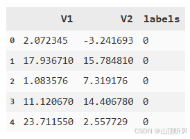

python 复制代码

#看一下 labels 里面有多少类别
pd.value_counts(y)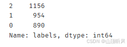

python 复制代码

#数据可视化
%matplotlib inline
from matplotlib import pyplot as plt
fig1 = plt.figure()
plt.scatter(X.loc[:,'V1'], X.loc[:,'V2'])
plt.title("un-labled data")
plt.xlabel('V1')
plt.ylabel('V2')
plt.show()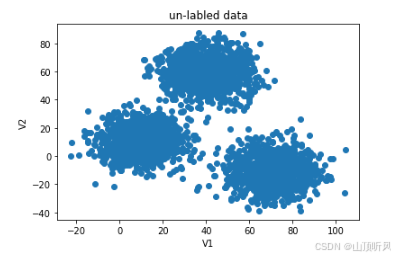

python 复制代码

fig1 = plt.figure()
label0 = plt.scatter(X.loc[:,'V1'][y==0], X.loc[:,'V2'][y==0])
label1 = plt.scatter(X.loc[:,'V1'][y==1], X.loc[:,'V2'][y==1])
label2 = plt.scatter(X.loc[:,'V1'][y==2], X.loc[:,'V2'][y==2])

plt.title("labeled data")
plt.xlabel('V1')
plt.ylabel('V2')
plt.legend((label0, label1, label2),('label0','label1','label2'))
plt.show()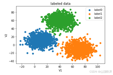

python 复制代码

print(X.shape, y.shape) # (3000, 2) (3000,)

Kmeans 算法（无监督）

创建模型并训练

python 复制代码

# set the model
from sklearn.cluster import KMeans
KM = KMeans(n_clusters = 3,  random_state = 0)
KM.fit(X)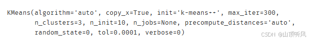

原始数据可视化

python 复制代码

centers = KM.cluster_centers_  # 三个中心点
fig3 = plt.figure()
#画原图
label0 = plt.scatter(X.loc[:,'V1'][y==0], X.loc[:,'V2'][y==0])
label1 = plt.scatter(X.loc[:,'V1'][y==1], X.loc[:,'V2'][y==1])
label2 = plt.scatter(X.loc[:,'V1'][y==2], X.loc[:,'V2'][y==2])

plt.title("labeled data")
plt.xlabel('V1')
plt.ylabel('V2')
plt.legend((label0, label1, label2),('label0','label1','label2'))

#展示中心点
plt.scatter(centers[:,0], centers[:,1])
plt.show()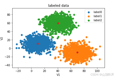

预测 V1=80,V2=60 数据类别

python 复制代码

# test data :V1 = 80, V2 = 60
y_predict_test = KM.predict([[80,60]])
print(y_predict_test) # [1]

python 复制代码

#predict based on training data
y_predict = KM.predict(X)
# 打印出预测数据的分布
print(pd.value_counts(y_predict),  pd.value_counts(y)) 
#发现与原始数据分布好像不太一样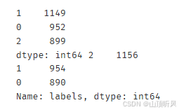

python 复制代码

#看下准确率
from sklearn.metrics import accuracy_score
accuracy = accuracy_score(y, y_predict)
print(accuracy) # 0.0023333333333333335, 可以看出准确率很低

预测数据与原数据一起展示

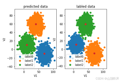
python 复制代码

#数据画出来看看哪里的问题
fig4 = plt.subplot(121)# 一行两列，画第一列

#画预测图==================================================
label0 = plt.scatter(X.loc[:,'V1'][y_predict==0], X.loc[:,'V2'][y_predict==0])
label1 = plt.scatter(X.loc[:,'V1'][y_predict==1], X.loc[:,'V2'][y_predict==1])
label2 = plt.scatter(X.loc[:,'V1'][y_predict==2], X.loc[:,'V2'][y_predict==2])
plt.title("predicted data")
plt.xlabel('V1')
plt.ylabel('V2')
plt.legend((label0, label1, label2),('label0','label1','label2'))
#展示中心点
plt.scatter(centers[:,0], centers[:,1])

#画原图==================================================
fig5 = plt.subplot(122)
label0 = plt.scatter(X.loc[:,'V1'][y==0], X.loc[:,'V2'][y==0])
label1 = plt.scatter(X.loc[:,'V1'][y==1], X.loc[:,'V2'][y==1])
label2 = plt.scatter(X.loc[:,'V1'][y==2], X.loc[:,'V2'][y==2])
plt.title("labled data")
plt.xlabel('V1')
plt.ylabel('V2')
plt.legend((label0, label1, label2),('label0','label1','label2'))
#展示中心点
plt.scatter(centers[:,0], centers[:,1])

plt.show() 
# 从下图可以看到，类别是区分出来了，但是类别名称不对；
# 这很正常，无监督式学习就是把类别区分出来至于取什么名称，那不一定
# 但是，如果已原数据的标签，可以将预结果的类别名称进行校正

类别校正

python 复制代码

# correct the results
y_corrected = []
for i in y_predict:
    if i == 0:
        y_corrected.append(1)
    elif i == 1:
        y_corrected.append(2)
    else:
        y_corrected.append(0)
print(pd.value_counts(y_corrected), pd.value_counts(y))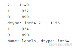

python 复制代码

# 看下校正后的准确率是多少
print(accuracy_score(y, y_corrected)) # 0.997

python 复制代码

y_corrected = np.array(y_corrected)
print(type(y_corrected)) # <class 'numpy.ndarray'>

校正后重新可视化

python 复制代码

#画出校正后的图形，y_predict 换成 y_corrected
fig6 = plt.subplot(121)# 一行两列，画第一列

#画预测图==================================================
label0 = plt.scatter(X.loc[:,'V1'][y_corrected==0], X.loc[:,'V2'][y_corrected==0])
label1 = plt.scatter(X.loc[:,'V1'][y_corrected==1], X.loc[:,'V2'][y_corrected==1])
label2 = plt.scatter(X.loc[:,'V1'][y_corrected==2], X.loc[:,'V2'][y_corrected==2])
plt.title("corrected data")
plt.xlabel('V1')
plt.ylabel('V2')
plt.legend((label0, label1, label2),('label0','label1','label2'))
#展示中心点
plt.scatter(centers[:,0], centers[:,1])

#画原图==================================================
fig7 = plt.subplot(122)
label0 = plt.scatter(X.loc[:,'V1'][y==0], X.loc[:,'V2'][y==0])
label1 = plt.scatter(X.loc[:,'V1'][y==1], X.loc[:,'V2'][y==1])
label2 = plt.scatter(X.loc[:,'V1'][y==2], X.loc[:,'V2'][y==2])
plt.title("labeled data")
plt.xlabel('V1')
plt.ylabel('V2')
plt.legend((label0, label1, label2),('label0','label1','label2'))
#展示中心点
plt.scatter(centers[:,0], centers[:,1])

plt.show()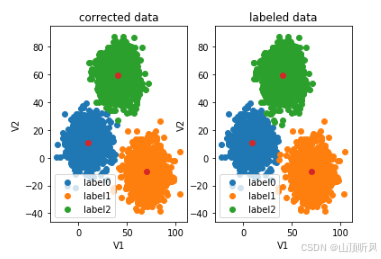

KNN　算法（有监督）

python 复制代码

#3、采用 KNN、Meanshift 算法，重复步骤 1-2
X.head()
y.head()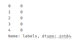

创建模型并训练

python 复制代码

#establish a KNN model(KNN 是 监督式)
from sklearn.neighbors import KNeighborsClassifier
KNN = KNeighborsClassifier(n_neighbors = 3)
KNN.fit(X, y)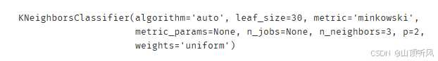

进行预测

复制代码

#predict based on the test data V1=80, V2=60
y_predict_knn_test = KNN.predict([[80,60]])
y_predict_knn = KNN.predict(X) # 训练数据使用 KNN的预测结果
print(y_predict_knn_test) # 结果：[2]
print('knn accureacy:', accuracy_score(y, y_predict_knn)) #knn accureacy: 1.0, 全部正确

python 复制代码

#打印出通过  KNN模型预测结果的分布，以及原来数据的分布
print(pd.value_counts(y_predict_knn), pd.value_counts(y)) # 可以看出完全一样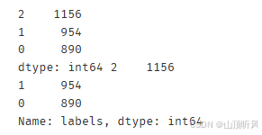

可视化

python 复制代码

#画图 KNN
fig8 = plt.subplot(121)# 一行两列，画第一列

#画预测图==================================================
label0 = plt.scatter(X.loc[:,'V1'][y_predict_knn==0], X.loc[:,'V2'][y_predict_knn==0])
label1 = plt.scatter(X.loc[:,'V1'][y_predict_knn==1], X.loc[:,'V2'][y_predict_knn==1])
label2 = plt.scatter(X.loc[:,'V1'][y_predict_knn==2], X.loc[:,'V2'][y_predict_knn==2])
plt.title("KNN results")
plt.xlabel('V1')
plt.ylabel('V2')
plt.legend((label0, label1, label2),('label0','label1','label2'))
#展示中心点
plt.scatter(centers[:,0], centers[:,1])

#画原图==================================================
fig9 = plt.subplot(122)
label0 = plt.scatter(X.loc[:,'V1'][y==0], X.loc[:,'V2'][y==0])
label1 = plt.scatter(X.loc[:,'V1'][y==1], X.loc[:,'V2'][y==1])
label2 = plt.scatter(X.loc[:,'V1'][y==2], X.loc[:,'V2'][y==2])
plt.title("labeled data")
plt.xlabel('V1')
plt.ylabel('V2')
plt.legend((label0, label1, label2),('label0','label1','label2'))
#展示中心点
plt.scatter(centers[:,0], centers[:,1])

plt.show()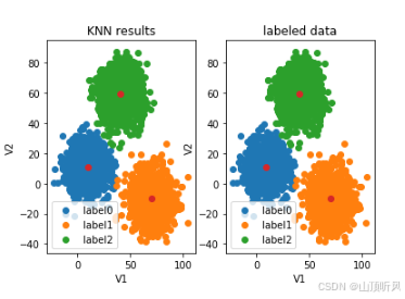

Meanshift 算法（无监督）

创建模型并训练

python 复制代码

#try the meanshift model,当只有数据，不知道能分成几个类别的时候使用，可以自动聚类出类别
from sklearn.cluster import MeanShift, estimate_bandwidth
# obtain the bandwidth
bw = estimate_bandwidth(X, n_samples = 500) # n_samples ：使用多少个样本点来估计带宽
print(bw) # 30.84663454820215, 带宽是 30
# 通过数据观察，横向X轴  150，纵向Y轴100，所以估出来 是 30 左右

python 复制代码

# establish the meanshift model( This is an un-supervised model.)
ms = MeanShift(bandwidth = bw)
ms.fit(X)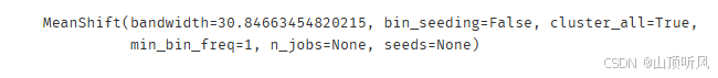

进行预测

python 复制代码

y_predict_ms = ms.predict(X)
print(pd.value_counts(y_predict_ms), pd.value_counts(y))# 自动归成了三类
#通过与原始数据的对比可以看出，与原始数据的类别名称不同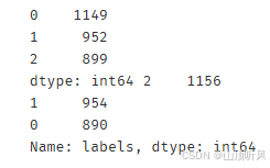

可视化

python 复制代码

#画图，meanshift
fig9 = plt.subplot(121)# 一行两列，画第一列

#画预测图==================================================
label0 = plt.scatter(X.loc[:,'V1'][y_predict_ms==0], X.loc[:,'V2'][y_predict_ms==0])
label1 = plt.scatter(X.loc[:,'V1'][y_predict_ms==1], X.loc[:,'V2'][y_predict_ms==1])
label2 = plt.scatter(X.loc[:,'V1'][y_predict_ms==2], X.loc[:,'V2'][y_predict_ms==2])
plt.title("ms results")
plt.xlabel('V1')
plt.ylabel('V2')
plt.legend((label0, label1, label2),('label0','label1','label2'))
#展示中心点
plt.scatter(centers[:,0], centers[:,1])

#画原图==================================================
fig10 = plt.subplot(122)
label0 = plt.scatter(X.loc[:,'V1'][y==0], X.loc[:,'V2'][y==0])
label1 = plt.scatter(X.loc[:,'V1'][y==1], X.loc[:,'V2'][y==1])
label2 = plt.scatter(X.loc[:,'V1'][y==2], X.loc[:,'V2'][y==2])
plt.title("labeled data")
plt.xlabel('V1')
plt.ylabel('V2')
plt.legend((label0, label1, label2),('label0','label1','label2'))
#展示中心点
plt.scatter(centers[:,0], centers[:,1])

plt.show() 
#通过图形发现，橙色部分是一样的，另两种类别反了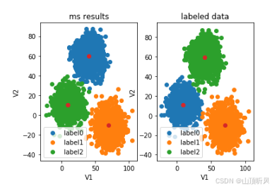

类别校正

python 复制代码

# correct the results
y_corrected_ms = []
for i in y_predict_ms:
    if i == 0:
        y_corrected_ms.append(2)
    elif i == 1:
          y_corrected_ms.append(1)
    elif i == 2:
        y_corrected_ms.append(0)
print(pd.value_counts(y_corrected_ms), pd.value_counts(y))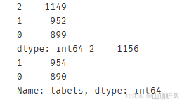

python 复制代码

# convert the results to numpy array
y_corrected_ms = np.array(y_corrected_ms)
print(type(y_corrected_ms))# <class 'numpy.ndarray'>

python 复制代码

#画预测图==================================================
label0 = plt.scatter(X.loc[:,'V1'][y_corrected_ms==0], X.loc[:,'V2'][y_corrected_ms==0])
label1 = plt.scatter(X.loc[:,'V1'][y_corrected_ms==1], X.loc[:,'V2'][y_corrected_ms==1])
label2 = plt.scatter(X.loc[:,'V1'][y_corrected_ms==2], X.loc[:,'V2'][y_corrected_ms==2])
plt.title("ms corrected results")
plt.xlabel('V1')
plt.ylabel('V2')
plt.legend((label0, label1, label2),('label0','label1','label2'))
#展示中心点
plt.scatter(centers[:,0], centers[:,1])

#画原图==================================================
fig12 = plt.subplot(122)
label0 = plt.scatter(X.loc[:,'V1'][y==0], X.loc[:,'V2'][y==0])
label1 = plt.scatter(X.loc[:,'V1'][y==1], X.loc[:,'V2'][y==1])
label2 = plt.scatter(X.loc[:,'V1'][y==2], X.loc[:,'V2'][y==2])
plt.title("labeled data")
plt.xlabel('V1')
plt.ylabel('V2')
plt.legend((label0, label1, label2),('label0','label1','label2'))
#展示中心点
plt.scatter(centers[:,0], centers[:,1])

plt.show()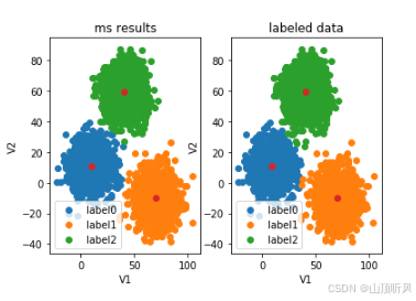

kmeans \ knn \ meanshift 总结

kmens \ meanshift: un-supervised, training data: X;

kmeans: need the category number;

meanshift:need to calculate the bandwidth;

knn: supervised: training data:X\y

分类算法 Kmeans、KNN、Meanshift 实战

任务

视频资料

数据准备

Kmeans 算法（无监督）

创建模型并训练

原始数据可视化

预测 V1=80,V2=60 数据类别

预测数据与原数据一起展示

类别校正

校正后重新可视化

KNN 算法（有监督）

创建模型并训练

进行预测

可视化

Meanshift 算法（无监督）

创建模型并训练

进行预测

可视化

类别校正

kmeans \ knn \ meanshift 总结

KNN　算法（有监督）