九、批量标准化
是一种广泛使用的神经网络正则化技术,对每一层的输入进行标准化,进行缩放和平移,目的是加速训练,提高模型稳定性和泛化能力,通常在全连接层或是卷积层之和,激活函数之前使用
核心思想
对每一批数据的通道进行标准化,解决内部协变量偏移
加速网络训练;运行使用更大的学习率;减少对初始化的依赖;提供轻微的正则化效果
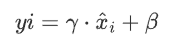
思路:在输入上执行标准化操作,学习两可训练的参数:缩放因子γ和偏移量β
批量标准化操作 在训练阶段和测试阶段行为是不同的。测试阶段没有mini_batch数据,无法直接计算当前batch的均值和方差,所以使用训练阶段计算的全局统量(均值和方差)进行标准化
1. 训练阶段的批量标准化
1.1 计算均值和方差
对于给定的神经网络层,输入 ,m是批次大小。我们计算该批次数据的均值和方差
均值
方差
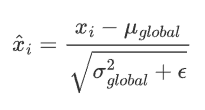
1.2 标准化
用计算得到的均值和方差对数据进行标准化,使得没个特征的均值为0,方差为1
标准化后的值
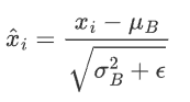
ε是很小的常数,防止除0
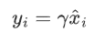
1.3 缩放和平移
标准化的数据通常会通过可训练的参数进行缩放和平移,以挥发模型的表达能力
缩放
平移
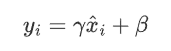
γ和β是在训练过程中学习到的参数,会随着网络的训练过程通过反向传播进行更新
1.4 更新全局统计量
指数移动平均更新全局均值和方差
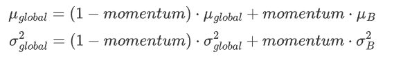
momentum是超变量,控制当前mini-batch统计量对全局统计量的贡献
它在0到1之间,控制mini-batch统计量的权重,在pytorch默认为0.1
与优化器中的momentum的区别
标准化中的:
更新全局统计量
控制当前mini-batch统计量对全局统计量的贡献
优化器中:
加速梯度下降,跳出局部最优
2.测试阶段的批量标准化
测试阶段没有mini-batch数据,所以通过EMA计算的全局统计量来进行标准化
测试阶段用全局统计量对输入数据进行标准化
对标准化后的数据进行缩放和平移
为什么用全局统计量
一致性:
-
在测试 阶段,输入数据通常是单个样本或少量样本 ,无法准确计算均值和方差。
-
使用全局统计量可以确保测试阶段的行为与训练阶段一致。
稳定性:
-
全局统计量是通过训练阶段的大量 mini-batch 数据计算得到的,能够更好地反映数据的整体分布。
-
使用全局统计量可以减少测试阶段的随机性 ,使模型的输出更加稳定。
效率:
- 在测试阶段,使用预先计算的全局统计量可以避免重复计算,提高效率。
3. 作用
3.1 缓解梯度问题
防止激活值过大或过小,避免激活函数的饱和,缓解梯度消失或爆炸
3.2 加速训练
输入值分布更稳定,提高学习训练的效率,加速收敛
3.3 减少过拟合
类似于正则化,有助于提高模型的泛化能力
避免对单一数据点的过度拟合
4. 函数说明
torch.nn.BatchNorm1d 是 PyTorch 中用于一维数据的批量标准化(Batch Normalization)模块。
torch.nn.BatchNorm1d(
    num_features,         # 输入数据的特征维度
    eps=1e-05,           # 用于数值稳定性的小常数
    momentum=0.1,        # 用于计算全局统计量的动量
    affine=True,         # 是否启用可学习的缩放和平移参数
    track_running_stats=True,  # 是否跟踪全局统计量
    device=None,         # 设备类型(如 CPU 或 GPU)
    dtype=None           # 数据类型
)
参数说明:
eps:用于数值稳定性的小常数 ,添加到方差的分母中,**防止除零错误。**默认值:1e-05
momentum:用于计算全局统计量 (均值和方差)的动量 。默认值:0.1,参考本节1.4
affine:是否启用可学习的缩放和平移参数(γ和 β)。如果 affine=True ,则模块会学习两个参数;如果 affine=False,则不学习参数 ,直接输出标准化后的值  。默认值:True
track_running_stats:是否跟踪全局统计量(均值和方差)。如果 track_running_stats=True,则在训练过程中计算并更新全局统计量,并在测试阶段使用这些统计量。如果 track_running_stats=False,则不跟踪全局统计量,每次标准化都使用当前 mini-batch 的统计量。默认值:True
4. 代码实现
import torch
from torch import nn
from matplotlib import pyplot as plt
from sklearn.datasets import make_circles
from sklearn.model_selection import train_test_split
from torch.nn import functional as F
from torch import optim
# 生成数据集:两个同心圆,内圈和外圈的点分别属于两个类别
x, y = make_circles(n_samples=2000, noise=0.1, factor=0.4, random_state=42)
# 转换为PyTorch张量
x = torch.tensor(x, dtype=torch.float32)
y = torch.tensor(y, dtype=torch.long)
# 划分训练集和测试集
x_train, x_test, y_train, y_test = train_test_split(x, y, test_size=0.3,
random_state=42)
# 可视化数据集
plt.scatter(x[:, 0], x[:, 1], c=y, cmap='coolwarm', edgecolors="k")
plt.show()
# 定义带批量归一化的神经网络
class NetWithBN(nn.Module):
def __init__(self):
super().__init__()
# 第一层全连接层,输入维度2,输出维度64
self.fc1 = nn.Linear(2, 64)
# 第一层批量归一化
self.bn1 = nn.BatchNorm1d(64)
# 第二层全连接层,输入维度64,输出维度32
self.fc2 = nn.Linear(64, 32)
# 第二层批量归一化
self.bn2 = nn.BatchNorm1d(32)
# 第三层全连接层,输入维度32,输出维度2(两个类别)
self.fc3 = nn.Linear(32, 2)
def forward(self, x):
# 前向传播:ReLU激活函数+批量归一化+全连接层
x = F.relu(self.bn1(self.fc1(x)))
x = F.relu(self.bn2(self.fc2(x)))
x = self.fc3(x)
return x
# 定义不带批量归一化的神经网络
class NetWithoutBN(nn.Module):
def __init__(self):
super().__init__()
# 第一层全连接层,输入维度2,输出维度64
self.fc1 = nn.Linear(2, 64)
# 第二层全连接层,输入维度64,输出维度32
self.fc2 = nn.Linear(64, 32)
# 第三层全连接层,输入维度32,输出维度2(两个类别)
self.fc3 = nn.Linear(32, 2)
def forward(self, x):
# 前向传播:ReLU激活函数+全连接层
x = F.relu(self.fc1(x))
x = F.relu(self.fc2(x))
x = self.fc3(x)
return x
# 定义训练函数
def train(model, x_train, y_train, x_test, y_test, name, lr=0.1, epoches=500):
# 定义交叉熵损失函数
criterion = nn.CrossEntropyLoss()
# 定义SGD优化器
optimizer = optim.SGD(model.parameters(), lr=lr)
# 用于记录训练损失和测试准确率
train_loss = []
test_acc = []
for epoch in range(epoches):
# 设置模型为训练模式
model.train()
# 前向传播
y_pred = model(x_train)
# 计算损失
loss = criterion(y_pred, y_train)
# 反向传播
optimizer.zero_grad()
loss.backward()
optimizer.step()
# 记录训练损失
train_loss.append(loss.item())
# 设置模型为评估模式
model.eval()
# 禁用梯度计算
with torch.no_grad():
# 前向传播
y_test_pred = model(x_test)
# 获取预测类别
_, pred = torch.max(y_test_pred, dim=1)
# 计算正确预测的数量
correct = (pred == y_test).sum().item()
# 计算测试准确率
test_acc.append(correct / len(y_test))
# 每100个epoch打印一次日志
if epoch % 100 == 0:
print(F"{name}|Epoch:{epoch},loss:{loss.item():.4f},acc:{test_acc[-1]:.4f}")
return train_loss, test_acc
# 创建带批量归一化的模型
model_bn = NetWithBN()
# 创建不带批量归一化的模型
model_nobn = NetWithoutBN()
# 训练带批量归一化的模型
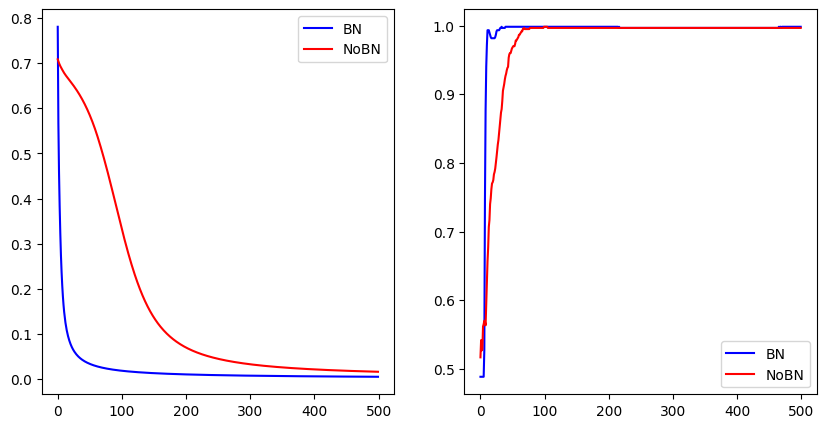
bn_train_loss, bn_test_acc = train(model_bn, x_train, y_train, x_test, y_test,
name="BN")
# 训练不带批量归一化的模型
nobn_train_loss, nobn_test_acc = train(model_nobn, x_train, y_train, x_test, y_test,
name="NoBN")
# 定义绘图函数
def plot(bn_train_loss, nobn_train_loss, bn_test_acc, nobn_test_acc):
# 创建绘图窗口
fig = plt.figure(figsize=(10, 5))
# 添加子图1:训练损失
ax1 = fig.add_subplot(1, 2, 1)
ax1.plot(bn_train_loss, "b", label="BN")
ax1.plot(nobn_train_loss, "r", label="NoBN")
ax1.legend()
# 添加子图2:测试准确率
ax2 = fig.add_subplot(1, 2, 2)
ax2.plot(bn_test_acc, "b", label="BN")
ax2.plot(nobn_test_acc, "r", label="NoBN")
ax2.legend()
# 显示图像
plt.show()
# 调用绘图函数
plot(bn_train_loss, nobn_train_loss, bn_test_acc, nobn_test_acc)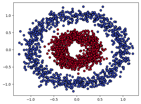
十、模型的保存和加载
1.标准网络模型构建
class MyModel(nn.Module):
    def __init__(self,input_size,output_size):
        super(MyModel,self).__init__()
        self.fc1 = nn.Linear(input_size,128)
        self.fc2 = nn.Linear(128,64)
        self.fc3 = nn.Linear(64,output_size)

    def forward(self,x):
        x = self.fc1(x)
        x = self.fc2(x)
        output = self.fc3(x)
        return output

model = MyModel(input_size=10,output_size = 2)
x  =torch.randn(5,10)

output = model(x)
2. 序列化模型对象
模型保存:
torch.save(obj, f, pickle_module=pickle, pickle_protocol=DEFAULT_PROTOCOL, _use_new_zipfile_serialization=True)
参数说明:
-
obj:要保存的对象,可以是模型、张量、字典等。
-
f:保存文件的路径或文件对象。可以是字符串(文件路径)或文件描述符。
-
pickle_module:用于序列化的模块,默认是 Python 的 pickle 模块。
-
pickle_protocol:pickle 模块的协议版本,默认是 DEFAULT_PROTOCOL(通常是最高版本)。
模型加载:
torch.load(f, map_location=None, pickle_module=pickle, **pickle_load_args)
参数说明:
-
f:文件路径或文件对象。可以是字符串(文件路径)或文件描述符。
-
map_location:指定加载对象的设备位置(如 CPU 或 GPU)。默认是 None,表示保持原始设备位置。例如:map_location=torch.device('cpu') 将对象加载到 CPU。
-
pickle_module:用于反序列化的模块,默认是 Python 的 pickle 模块。
-
pickle_load_args:传递给 pickle_module.load() 的额外参数。
import torch
import torch.nn as nn
import pickleclass MyModel(nn.Module):
def init(self,input_size,output_size):
super(MyModel,self).init()
self.fc1 = nn.Linear(input_size,output_size,128)
self.fc2 = nn.Linear(128,64)
self.fc3 = nn.Linear(64,output_size)def forward(self,x): x = self.fc1(x) x = self.fc2(x) output = self.fc3(x) return outputdef test001():
model = MyModel(input_size=128,output_size=32)
torch.save(model,"model.pkl",pickle_module=pickle,pickle_protocol=2)def test002():
model = torch.load("model.pkl",map_location = "cpu",pickle_module=pickle)
print(model)test001()
test002()
.pkl是二进制文件,内容是通过pickle模块化序列的python对象。可能存在兼容问题(python2,3的区别)
.pth是二进制文件,序列化的pytorch模型或张量。
3. 模型保存参数
import torch
import torch.nn as nn
import torch.optim as optim
import pickle
class MyModle(nn.Module):
def __init__(self,input_size,output_size):
super(MyModle,self).__init__()
self.fc1 = nn.Linear(input_size,128)
self.fc2 = nn.Linear(128,64)
self.fc3 = nn.Linear(64,output_size)
  def forward(self,x):
      x = self.fc1(x)
      x = self.fc2(x)
      output = self.fc3(x)
      return output
def test003():
model = MyModle(input_size=128,output_size=32)
optimizer = optim.SGD(model.parameters(),lr = 0.01)
save_dict = {
"init_params":{
"input_size":128,
"output_size":32,
},
"accuracy":0.99,
"model_state_dict":model.state_dict(),
"optimizer_state_dict":optimizer.state_dict(),
}
torch.save(save_dict,"model_dict.pth")
def test004():
save_dict = torch.load("model_dict.pth")
model = MyModle(
input_size = save_dict["init_params"]["input_size"],
output_size = save_dict["init_params"]["output_size"],
)
model.load_state_dict(save_dict["model_state_dict"])
optimizer = optim.SGD(model.parameters(),lr = 0.01)
optimizer.load_state_dict(save_dict["optimizer_state_dict"])
print(save_dict["accuracy"])
print(model)
test003()
test004()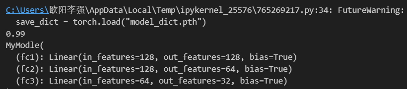
推理时加载模型参数简单如下:
# 保存模型状态字典 torch.save(model.state_dict(), 'model.pth') # 加载模型状态字典 model = MyModel(128, 32) model.load_state_dict(torch.load('model.pth'))