目录
超参数搜索的3D曲面可视化
python
## 超参数搜索的3D曲面可视化

import numpy as np
import matplotlib.pyplot as plt
from mpl_toolkits.mplot3d import Axes3D
from sklearn.datasets import make_regression
from sklearn.ensemble import RandomForestRegressor
from sklearn.model_selection import cross_val_score
from sklearn.metrics import mean_squared_error

# 回归数据集
X, y = make_regression(n_samples=1000, n_features=20, noise=0.1, random_state=42)

# 定义要搜索的超参数范围
n_estimators_range = np.linspace(10, 200, 10).astype(int)
max_depth_range = np.linspace(3, 15, 10).astype(int)

# 创建网格用于存储结果
n_estimators_grid, max_depth_grid = np.meshgrid(n_estimators_range, max_depth_range)
mse_grid = np.zeros_like(n_estimators_grid, dtype=float)

# 遍历所有参数组合
for i in range(len(n_estimators_range)):
    for j in range(len(max_depth_range)):
        model = RandomForestRegressor(
            n_estimators=n_estimators_range[i],
            max_depth=max_depth_range[j],
            random_state=42
        )
        scores = cross_val_score(model, X, y, cv=5,
                               scoring='neg_mean_squared_error')
        mse_grid[j, i] = -scores.mean()  # 转换为正MSE

# 创建3D图形
fig = plt.figure(figsize=(12, 8))
ax = fig.add_subplot(111, projection='3d')

# 绘制曲面
surf = ax.plot_surface(n_estimators_grid, max_depth_grid, mse_grid,
                      cmap='viridis', edgecolor='none', alpha=0.8)

# 添加等高线投影
cset = ax.contourf(n_estimators_grid, max_depth_grid, mse_grid,
                  zdir='z', offset=mse_grid.min()-0.1, cmap='viridis', alpha=0.5)

# 标记最佳点
min_idx = np.unravel_index(np.argmin(mse_grid), mse_grid.shape)
ax.scatter(n_estimators_grid[min_idx], max_depth_grid[min_idx], mse_grid[min_idx],
          color='red', s=100, label=f'Best (MSE={mse_grid[min_idx]:.2f})')

# 设置标签和标题
ax.set_xlabel('Number of Estimators')
ax.set_ylabel('Max Depth')
ax.set_zlabel('Mean Squared Error')
ax.set_title('Random Forest Hyperparameter Tuning (3D Surface)')
ax.legend()

# 添加颜色条
fig.colorbar(surf, shrink=0.5, aspect=5)

# 调整视角
ax.view_init(elev=30, azim=45)

plt.tight_layout()
plt.show()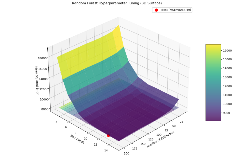
交互式3D可视化
python
## 交互式3D可视化
import plotly.graph_objects as go
from plotly.subplots import make_subplots
import numpy as np
import matplotlib.pyplot as plt
from mpl_toolkits.mplot3d import Axes3D
from sklearn.datasets import make_regression
from sklearn.ensemble import RandomForestRegressor
from sklearn.model_selection import cross_val_score
from sklearn.metrics import mean_squared_error

# 回归数据集
X, y = make_regression(n_samples=1000, n_features=20, noise=0.1, random_state=42)

# 定义要搜索的超参数范围
n_estimators_range = np.linspace(10, 200, 10).astype(int)
max_depth_range = np.linspace(3, 15, 10).astype(int)

# 创建网格用于存储结果
n_estimators_grid, max_depth_grid = np.meshgrid(n_estimators_range, max_depth_range)
mse_grid = np.zeros_like(n_estimators_grid, dtype=float)

# 创建交互式3D图形
fig = go.Figure(data=[go.Surface(
    z=mse_grid,
    x=n_estimators_range,
    y=max_depth_range,
    colorscale='Viridis',
    opacity=0.8,
    contours={
        "z": {"show": True, "start": mse_grid.min(), "end": mse_grid.max(),
              "size": (mse_grid.max()-mse_grid.min())/10}
    }
)])
min_idx = np.unravel_index(np.argmin(mse_grid), mse_grid.shape)
# 标记最佳点
fig.add_trace(go.Scatter3d(
    x=[n_estimators_range[min_idx[1]]],
    y=[max_depth_range[min_idx[0]]],
    z=[mse_grid.min()],
    mode='markers',
    marker=dict(size=10, color='red'),
    name=f'Best (MSE={mse_grid.min():.2f})'
))

# 设置布局
fig.update_layout(
    title='Random Forest Hyperparameter Tuning (Interactive 3D)',
    scene=dict(
        xaxis_title='Number of Estimators',
        yaxis_title='Max Depth',
        zaxis_title='Mean Squared Error',
        camera=dict(
            eye=dict(x=1.5, y=1.5, z=0.8)  # 调整初始视角
        )
    ),
    width=800,
    height=600,
    margin=dict(r=20, l=10, b=10, t=50)
)

fig.show()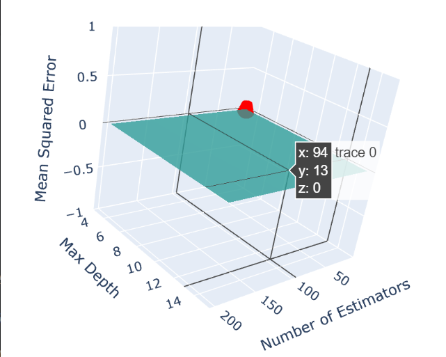
神经网络学习率的3D可视化
python
## 神经网络学习率的3D可视化
import tensorflow as tf
from tensorflow.keras.models import Sequential
from tensorflow.keras.layers import Dense
from tensorflow.keras.wrappers.scikit_learn import KerasRegressor
import numpy as np
import matplotlib.pyplot as plt
from sklearn.datasets import make_regression
from sklearn.model_selection import cross_val_score


# 准备数据
X, y = make_regression(n_samples=1000, n_features=20, noise=0.1, random_state=42)

# 定义参数网格
learning_rates = np.logspace(-4, -1, 10)
batch_sizes = [16, 32, 64, 128, 256]

# 创建网格
lr_grid, bs_grid = np.meshgrid(learning_rates, batch_sizes)
mse_grid = np.zeros_like(lr_grid, dtype=float)

# 构建模型函数
def build_model(lr=0.001):
    model = Sequential([
        Dense(64, activation='relu', input_shape=(20,)),
        Dense(32, activation='relu'),
        Dense(1)
    ])
    model.compile(optimizer=tf.keras.optimizers.Adam(learning_rate=lr),
                 loss='mse')
    return model

# 遍历参数组合
for i in range(len(learning_rates)):
    for j in range(len(batch_sizes)):
        model = KerasRegressor(build_fn=lambda lr=learning_rates[i]: build_model(lr),
                             epochs=20, batch_size=batch_sizes[j], verbose=0)
        scores = cross_val_score(model, X, y, cv=3,
                               scoring='neg_mean_squared_error')
        mse_grid[j, i] = -scores.mean()

# 创建3D图形
fig = plt.figure(figsize=(12, 8))
ax = fig.add_subplot(111, projection='3d')

# 绘制曲面 (使用对数坐标)
surf = ax.plot_surface(np.log10(lr_grid), bs_grid, mse_grid,
                      cmap='plasma', edgecolor='none', alpha=0.8)

# 标记最佳点
min_idx = np.unravel_index(np.argmin(mse_grid), mse_grid.shape)
ax.scatter(np.log10(lr_grid[min_idx]), bs_grid[min_idx], mse_grid[min_idx],
          color='red', s=100, label=f'Best (MSE={mse_grid[min_idx]:.2f})')

# 设置标签和标题
ax.set_xlabel('log10(Learning Rate)')
ax.set_ylabel('Batch Size')
ax.set_zlabel('Mean Squared Error')
ax.set_title('Neural Network Hyperparameter Tuning (3D Surface)')
ax.legend()

# 添加颜色条
fig.colorbar(surf, shrink=0.5, aspect=5)

# 调整视角
ax.view_init(elev=30, azim=45)

plt.tight_layout()
plt.show()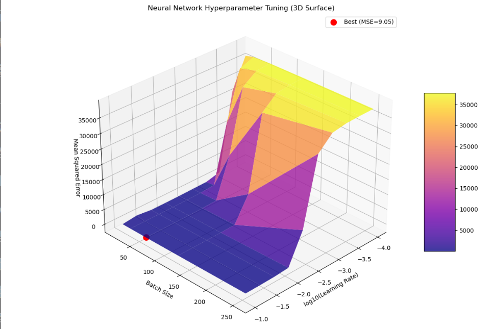
SVM超参数的3D决策边界可视化
python
## SVM超参数的3D决策边界可视化
from sklearn.svm import SVC
from sklearn.datasets import make_classification
from mlxtend.plotting import plot_decision_regions
import matplotlib.pyplot as plt
import numpy as np
# 生成分类数据
X, y = make_classification(n_samples=200, n_features=2, n_redundant=0,
n_informative=2, random_state=42, n_clusters_per_class=1)
# 定义参数网格
C_range = np.logspace(-2, 2, 5)
gamma_range = np.logspace(-3, 1, 5)
# 创建3D图形
fig = plt.figure(figsize=(25, 25))
# 遍历参数组合并绘制决策边界
for i, C in enumerate(C_range):
for j, gamma in enumerate(gamma_range):
ax = fig.add_subplot(len(C_range), len(gamma_range), i * len(gamma_range) + j + 1,
projection='3d')
# 训练SVM模型
model = SVC(C=C, gamma=gamma, probability=True)
model.fit(X, y)
# 创建网格点
x_min, x_max = X[:, 0].min() - 1, X[:, 0].max() + 1
y_min, y_max = X[:, 1].min() - 1, X[:, 1].max() + 1
xx, yy = np.meshgrid(np.linspace(x_min, x_max, 50),
np.linspace(y_min, y_max, 50))
# 计算决策函数值
Z = model.decision_function(np.c_[xx.ravel(), yy.ravel()])
Z = Z.reshape(xx.shape)
# 绘制3D决策边界
ax.plot_surface(xx, yy, Z, cmap='coolwarm', alpha=0.8)
ax.scatter(X[:, 0], X[:, 1], y, c=y, cmap='coolwarm', s=20, edgecolors='k')
ax.set_title(f'C={C:.2f}, γ={gamma:.2f}')
ax.set_xlabel('Feature 1')
ax.set_ylabel('Feature 2')
ax.set_zlabel('Decision Function')
plt.tight_layout()
plt.show()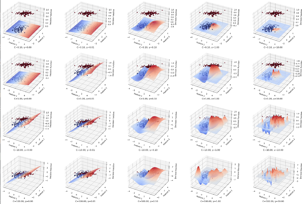 超参数优化的3D动画
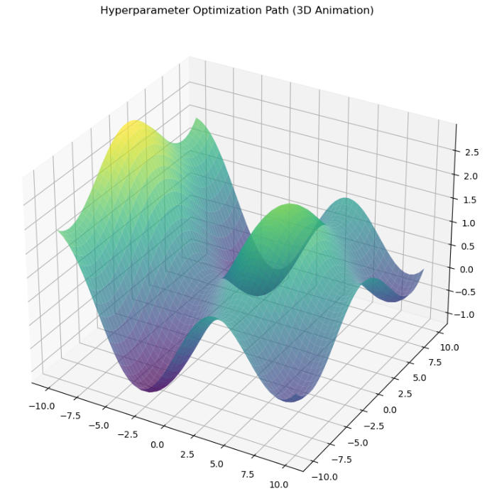
python
## 超参数优化的3D动画

from matplotlib.animation import FuncAnimation
from scipy.optimize import minimize
import matplotlib.pyplot as plt
import numpy as np


# 定义目标函数 (模拟的损失函数)
def objective(params):
    x, y = params
    return np.sin(x / 2) + np.cos(y / 3) + (x ** 2 + y ** 2) / 100


# 准备数据
x = np.linspace(-10, 10, 50)
y = np.linspace(-10, 10, 50)
X, Y = np.meshgrid(x, y)
Z = np.zeros_like(X)
for i in range(len(x)):
    for j in range(len(y)):
        Z[j, i] = objective([x[i], y[j]])

# 优化过程
initial_guess = [8, 8]
path = [initial_guess]


def store_path(params):
    path.append(params)
    return objective(params)


result = minimize(store_path, initial_guess, method='BFGS',
                  options={'disp': True})

# 创建3D图形
fig = plt.figure(figsize=(10, 8))
ax = fig.add_subplot(111, projection='3d')

# 绘制曲面
surf = ax.plot_surface(X, Y, Z, cmap='viridis', alpha=0.7)

# 初始点
point, = ax.plot([], [], [], 'ro', markersize=10)
line, = ax.plot([], [], [], 'r-', linewidth=2)


# 初始化函数
def init():
    point.set_data([], [])
    point.set_3d_properties([])
    line.set_data([], [])
    line.set_3d_properties([])
    return point, line


# 更新函数
def update(frame):
    x_data = [p[0] for p in path[:frame]]
    y_data = [p[1] for p in path[:frame]]
    z_data = [objective(p) for p in path[:frame]]

    point.set_data([x_data[-1]], [y_data[-1]])
    point.set_3d_properties([z_data[-1]])

    line.set_data(x_data, y_data)
    line.set_3d_properties(z_data)

    ax.view_init(elev=30, azim=frame / 2)  # 缓慢旋转视角

    return point, line


# 创建动画
ani = FuncAnimation(fig, update, frames=len(path), init_func=init,
                    interval=300, blit=True, repeat_delay=1000)

plt.title('Hyperparameter Optimization Path (3D Animation)')
plt.tight_layout()
plt.show()