前言
提醒:
文章内容为方便作者自己后日复习与查阅而进行的书写与发布,其中引用内容都会使用链接表明出处(如有侵权问题,请及时联系)。
其中内容多为一次书写,缺少检查与订正,如有问题或其他拓展及意见建议,欢迎评论区讨论交流。
内容由AI辅助生成,仅经笔者审核整理,请甄别食用。
文章目录
- 前言
-
-
- [一、世代距离(GD)------ 聚焦收敛性的度量](#一、世代距离(GD)—— 聚焦收敛性的度量)
-
- [1. 核心目标](#1. 核心目标)
- [2. 数学公式与拆解](#2. 数学公式与拆解)
- [3. 物理意义](#3. 物理意义)
- [4. 可视化示例](#4. 可视化示例)
- [二、反转世代距离(IGD)------ 收敛+多样性双维度度量](#二、反转世代距离(IGD)—— 收敛+多样性双维度度量)
-
- [1. 核心目标](#1. 核心目标)
- [2. 数学公式与拆解](#2. 数学公式与拆解)
- [3. 物理意义](#3. 物理意义)
- [4. 可视化示例](#4. 可视化示例)
- [三、GD vs IGD ------ 核心差异与适用场景](#三、GD vs IGD —— 核心差异与适用场景)
- 五、总结
-
一、世代距离(GD)------ 聚焦收敛性的度量
1. 核心目标
衡量近似解集 A A A到真实帕累托前沿 P F PF PF的"收敛差距",即算法生成的解是否足够接近最优前沿。
2. 数学公式与拆解
G D = 1 ∣ A ∣ ( ∑ i = 1 ∣ A ∣ dis ( a i , P F ′ ) p ) 1 p GD = \frac{1}{|A|} \left( \sum_{i=1}^{|A|} \text{dis}(a_i, PF')^p \right)^{\frac{1}{p}} GD=∣A∣1 i=1∑∣A∣dis(ai,PF′)p p1
- 符号定义 :
- ∣ A ∣ |A| ∣A∣:近似解集 A A A的规模(解的数量,如算法最终保留的非支配解个数);
- P F ′ PF' PF′:真实帕累托前沿 P F PF PF的简化子集 (因 P F PF PF可能连续,需采样离散点集,保证计算可行性);
- dis ( a i , P F ′ ) \text{dis}(a_i, PF') dis(ai,PF′):近似解 a i a_i ai到 P F ′ PF' PF′的最小欧氏距离 ,即 a i a_i ai与 P F ′ PF' PF′中所有点的距离最小值,公式为:
dis ( a i , P F ′ ) = min p ∈ P F ′ ∑ m = 1 M ( a i , m − p m ) 2 \text{dis}(a_i, PF') = \min_{p \in PF'} \sqrt{\sum_{m=1}^M (a_{i,m} - p_m)^2} dis(ai,PF′)=p∈PF′minm=1∑M(ai,m−pm)2
( M M M是目标维度, a i , m a_{i,m} ai,m是 a i a_i ai的第 m m m个目标值, p m p_m pm是 P F ′ PF' PF′中点 p p p的第 m m m个目标值); - p p p:范数参数 ,通常取 p = 2 p=2 p=2(计算均方根距离,突出离群点;取 p = 1 p=1 p=1则为平均距离)。
3. 物理意义
- 收敛性 : G D GD GD越小,说明近似解整体越贴近真实帕累托前沿,算法的收敛性越好;
- 局限性 :仅关注"解是否够好",不衡量"解是否覆盖前沿"(比如所有解扎堆在前沿某区域, G D GD GD也可能很小,但多样性差)。
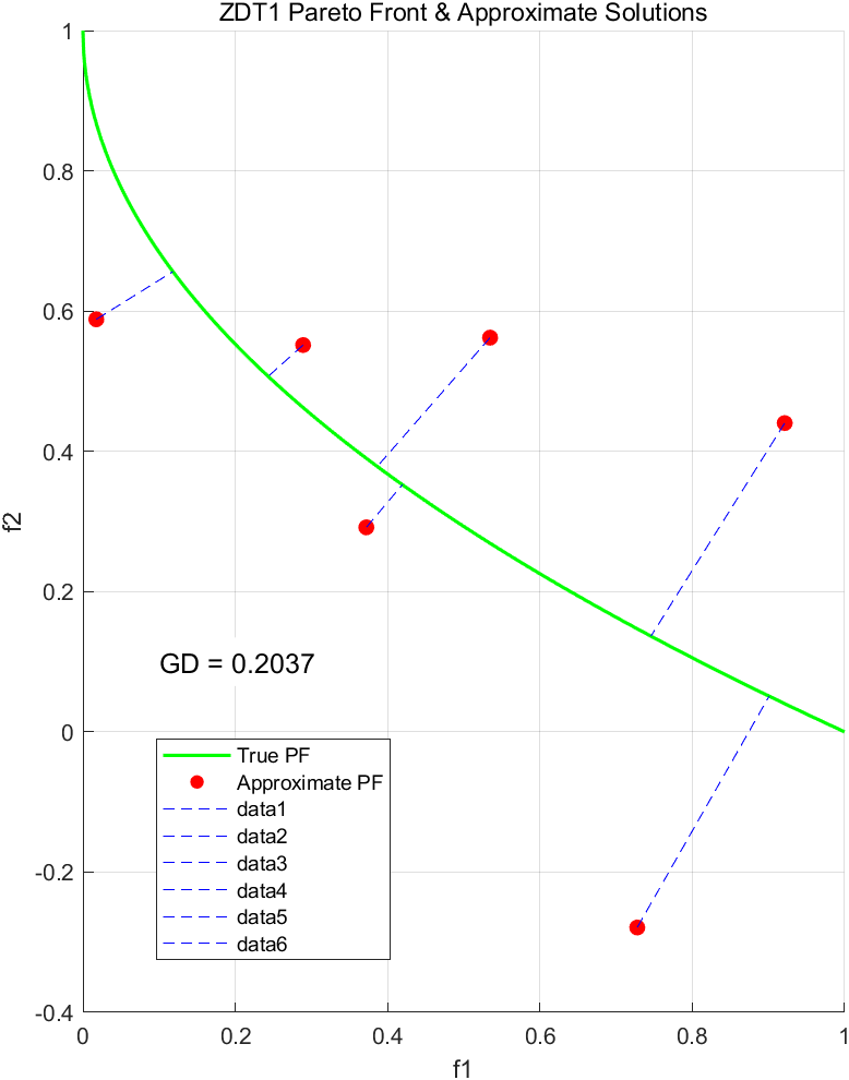
4. 可视化示例
二维可视化代码以及运行结果:
matlab
clc; clear; close all;

%% 设置参数
N_true = 1000;   % 真实帕累托前沿点数(少量)
N_approx = 6;  % 近似前沿点数(更少)

%% 生成 ZDT1 的真实帕累托前沿
x_true = linspace(0,1,N_true)';
f1_true = x_true;
f2_true = 1 - sqrt(x_true);
true_pf = [f1_true, f2_true];

%% 模拟近似帕累托前沿(稍微偏离真实解)
rng(1);
x_approx = linspace(0.05, 0.95, N_approx)' + 0.05*randn(N_approx,1);
x_approx = min(max(x_approx,0),1);
f1_approx = x_approx;
f2_approx = 1 - sqrt(x_approx) + 0.5*randn(N_approx,1);
approx_pf = [f1_approx, f2_approx];

%% 可视化解集
figure; hold on; grid on;
plot(f1_true, f2_true, 'g-', 'LineWidth', 1.5);
scatter(f1_approx, f2_approx, 50, 'r', 'filled');
legend('True PF', 'Approximate PF', 'Location','best');
xlabel('f1'); ylabel('f2');
title('ZDT1 Pareto Front & Approximate Solutions');

%% 可视化计算过程 + GD
distances = zeros(N_approx, 1);
for i = 1:N_approx
    % 当前近似点
    p = approx_pf(i, :);
    % 到所有真实点的欧式距离
    d = vecnorm(true_pf - p, 2, 2);
    [min_dist, idx] = min(d);
    distances(i) = min_dist;

    % 可视化该点与最近真实点之间的距离线
    q = true_pf(idx, :);
    plot([p(1), q(1)], [p(2), q(2)], 'b--'); % 蓝色虚线表示距离
end

% 计算 GD
GD = mean(distances);
text(0.1, 0.1, ['GD = ', num2str(GD, '%.4f')], 'FontSize', 12, 'BackgroundColor', 'w');
运行结果
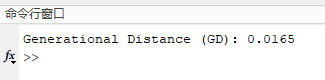
三维可视化代码以及运行结果:
matlab
clc; clear; close all;

%% 参数设置
M = 3;                  % 目标数(三维)
refPointsNum = 20000;    % 参考前沿点数量(大量)
approxPointsNum = 50;   % 近似解数量(较少)
disturbance = 0.1;     % 扰动大小(控制近似解与参考点距离)

%% 生成参考帕累托前沿(单位球面均匀分布点)
theta1 = rand(refPointsNum,1)*pi/2;
theta2 = rand(refPointsNum,1)*pi/2;

f1 = cos(theta1).*cos(theta2);
f2 = cos(theta1).*sin(theta2);
f3 = sin(theta1);
RefFront = [f1 f2 f3];
RefFront = RefFront ./ vecnorm(RefFront,2,2);

%% 生成少量近似解,扰动控制在disturbance范围内
idxSample = randsample(refPointsNum, approxPointsNum);
PopObjs = RefFront(idxSample,:) + disturbance*randn(approxPointsNum, M);
PopObjs = max(PopObjs, 0);          % 保持非负
% PopObjs = PopObjs ./ vecnorm(PopObjs,2,2); % 归一化,保证落在球面附近
PopObjs = PopObjs;
%% 计算世代距离(GD)
distances = zeros(approxPointsNum,1);
for i = 1:approxPointsNum
    d = sqrt(sum((RefFront - PopObjs(i,:)).^2, 2));
    distances(i) = min(d);
end
GD = sqrt(sum(distances.^2))/approxPointsNum;

fprintf('Generational Distance (GD): %.4f\n', GD);

%% 可视化
figure; hold on; grid on; axis equal;
scatter3(RefFront(:,1), RefFront(:,2), RefFront(:,3), 10, 'g', 'filled');
scatter3(PopObjs(:,1), PopObjs(:,2), PopObjs(:,3), 60, 'r', 'filled');

% 画距离连线
for i = 1:approxPointsNum
    d = sqrt(sum((RefFront - PopObjs(i,:)).^2, 2));
    [~, idx] = min(d);
    plot3([PopObjs(i,1) RefFront(idx,1)], ...
          [PopObjs(i,2) RefFront(idx,2)], ...
          [PopObjs(i,3) RefFront(idx,3)], 'b--');
end

xlabel('Objective 1'); ylabel('Objective 2'); zlabel('Objective 3');
title(sprintf('DTLZ2 3-Objective Problem - GD=%.4f', GD));
legend('Reference Pareto Front','Approximate Solutions','Distance Lines');
view(45,30);
运行结果
二、反转世代距离(IGD)------ 收敛+多样性双维度度量
1. 核心目标
同时衡量近似解集 A A A的收敛性(贴近 P F PF PF)和多样性(覆盖 P F PF PF),即解是否"又好又全"。
2. 数学公式与拆解
I G D = 1 ∣ P F ′ ∣ ( ∑ i = 1 ∣ P F ′ ∣ dis ( p i , A ) p ) 1 p IGD = \frac{1}{|PF'|} \left( \sum_{i=1}^{|PF'|} \text{dis}(p_i, A)^p \right)^{\frac{1}{p}} IGD=∣PF′∣1 i=1∑∣PF′∣dis(pi,A)p p1
- 符号定义 :
- ∣ P F ′ ∣ |PF'| ∣PF′∣:真实帕累托前沿子集 P F ′ PF' PF′的规模(采样点数量,需均匀覆盖 P F PF PF);
- dis ( p i , A ) \text{dis}(p_i, A) dis(pi,A): P F ′ PF' PF′中的点 p i p_i pi到近似解集 A A A的最小欧氏距离 (即 p i p_i pi与 A A A中最近点的距离),公式为:
dis ( p i , A ) = min a ∈ A ∑ m = 1 M ( p i , m − a m ) 2 \text{dis}(p_i, A) = \min_{a \in A} \sqrt{\sum_{m=1}^M (p_{i,m} - a_m)^2} dis(pi,A)=a∈Aminm=1∑M(pi,m−am)2
( p i , m p_{i,m} pi,m是 p i p_i pi的第 m m m个目标值, a m a_m am是 A A A中点 a a a的第 m m m个目标值); - p p p:同 GD,通常取 p = 2 p=2 p=2。
3. 物理意义
- 收敛性 : I G D IGD IGD越小,说明 P F ′ PF' PF′到 A A A的距离越小, A A A越贴近 P F PF PF;
- 多样性 :若 A A A分布稀疏(比如只覆盖 P F PF PF的局部区域),则 P F ′ PF' PF′中远离 A A A的点会使 I G D IGD IGD增大,因此 I G D IGD IGD能惩罚"解分布不均"的问题;
- 优势:相比 GD,IGD 更全面,能同时反映"解的质量"和"解的覆盖性"。
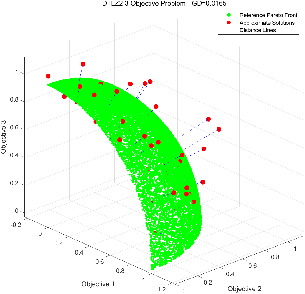
4. 可视化示例
二维可视化代码以及运行结果:
matlab
clc;
clear;
close all;

%% 设置参数
N_true = 100;   % 真实帕累托前沿点数
N_approx = 6;    % 近似前沿点数
perturbation_size = 0.5;  % 扰动大小

%% 生成 ZDT1 的真实帕累托前沿
x_true = linspace(0, 1, N_true)';
f1_true = x_true;
f2_true = 1 - sqrt(x_true);
true_pf = [f1_true, f2_true];

%% 模拟近似帕累托前沿(稍微偏离真实解)
rng(1);
x_approx = linspace(0.05, 0.95, N_approx)' + perturbation_size * randn(N_approx, 1);
x_approx = min(max(x_approx, 0), 1);  % 限制在 [0, 1] 范围内
f1_approx = x_approx;
f2_approx = 1 - sqrt(x_approx) + perturbation_size * randn(N_approx, 1);
approx_pf = [f1_approx, f2_approx];

%% 可视化解集
figure; hold on; grid on;
plot(f1_true, f2_true, 'g-', 'LineWidth', 1.5, 'DisplayName', 'True PF');  % 绘制真实帕累托前沿
scatter(f1_approx, f2_approx, 50, 'r', 'filled', 'DisplayName', 'Approximate PF');  % 绘制近似前沿
xlabel('f1'); ylabel('f2');
title('ZDT1 Pareto Front & Approximate Solutions');

%% 计算 IGD
distances = zeros(N_true, 1);  % 存储每个真实点到最近近似点的距离
for i = 1:N_true
    % 当前真实点
    p = true_pf(i, :);
    % 到所有近似点的欧式距离
    d = vecnorm(approx_pf - p, 2, 2);
    % 记录最近的距离
    distances(i) = min(d);
end

% 计算 IGD
IGD = mean(distances);
% 可视化计算过程
for i = 1:N_true
    % 当前真实点
    p = true_pf(i, :);
    % 到所有近似点的欧式距离
    d = vecnorm(approx_pf - p, 2, 2);
    [min_dist, idx] = min(d);  % 找到最近的近似点

    % 可视化该真实点与最近近似点之间的距离线
    q = approx_pf(idx, :);
    plot([p(1), q(1)], [p(2), q(2)], 'b--'); % 蓝色虚线表示距离
end

% 显示 IGD
text(0.1, 0.1, ['IGD = ', num2str(IGD, '%.4f')], 'FontSize', 12, 'BackgroundColor', 'w');

% 添加图例,显示'非数据'标签
legend('True PF', 'Approximate PF', 'Location', 'best');
hold off;
运行结果
三维可视化代码以及运行结果:
matlab
clc; clear; close all;
%% 参数配置
M = 3; % 目标函数维度(三维)
refPointsNum = 50; % 参考帕累托前沿点数量
approxPointsNum = 8; % 近似解数量
disturbance = 0.08; % 扰动大小(控制近似解质量)
%% 生成DTLZ2参考帕累托前沿(PF)
theta1 = linspace(0, pi/2, sqrt(refPointsNum))';
theta2 = linspace(0, pi/2, sqrt(refPointsNum));
[Theta1, Theta2] = meshgrid(theta1, theta2);
% 计算目标函数值
f1 = cos(Theta1) .* cos(Theta2);
f2 = cos(Theta1) .* sin(Theta2);
f3 = sin(Theta1);
% 转换为向量形式并归一化
PF = [f1(:) f2(:) f3(:)];
PF = PF ./ vecnorm(PF, 2, 2); % 单位球面归一化
%% 生成近似解(A)
idxSample = randsample(size(PF, 1), approxPointsNum);
A = PF(idxSample, :) + disturbance * randn(approxPointsNum, M);
A = max(min(A, 1), 0); % 限制在合理范围
%% 计算反转世代距离(IGD)
% IGD公式:IGD = (1/|PF|) * Σ(min距离(PF_i, A))
% 物理意义:每个参考点到最近近似解的平均距离(PF→A)
igd_distances = zeros(size(PF, 1), 1);
for i = 1:size(PF, 1)
% 计算PF中每个点到所有近似解的距离
dists = sqrt(sum((A - PF(i, :)).^2, 2));
igd_distances(i) = min(dists); % 取最近距离
end
IGD = mean(igd_distances);
%% 计算世代距离(GD)
% GD公式:GD = (1/|A|) * Σ(min距离(A_j, PF))
% 物理意义:每个近似解到最近参考点的平均距离(A→PF)
gd_distances = zeros(size(A, 1), 1);
for j = 1:size(A, 1)
% 计算每个近似解到所有PF点的距离
dists = sqrt(sum((PF - A(j, :)).^2, 2));
gd_distances(j) = min(dists); % 取最近距离
end
GD = mean(gd_distances);
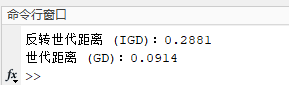
%% 输出结果
fprintf('反转世代距离 (IGD):%.4f\n', IGD);
fprintf('世代距离 (GD):%.4f\n', GD);
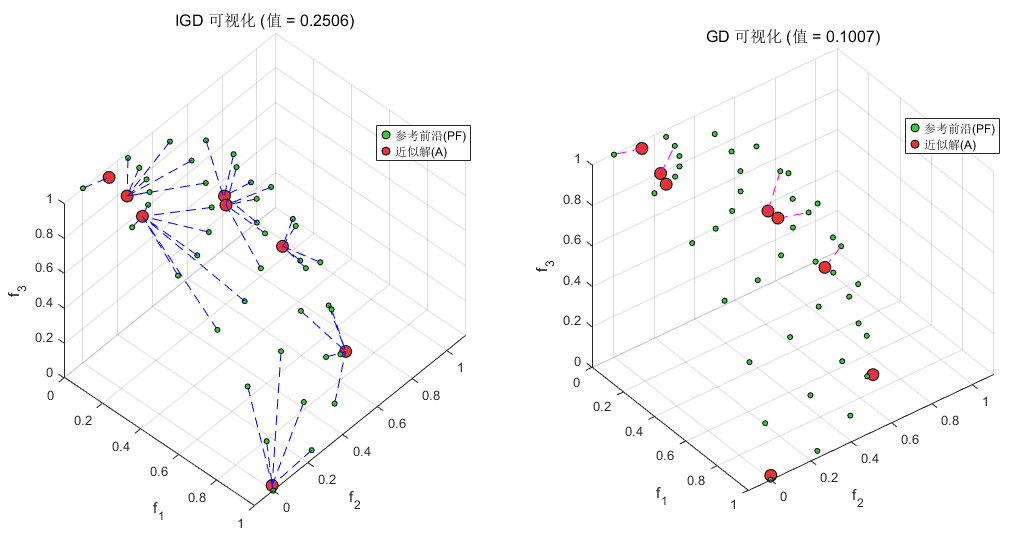
%% 可视化对比
figure('Position', [100, 100, 1200, 600], 'Color', 'w');
% 左侧:IGD可视化(PF→A的距离)
subplot(1, 2, 1); hold on; grid on; axis equal;
scatter3(PF(:, 1), PF(:, 2), PF(:, 3), 15, [0.2 0.8 0.2], ...
'filled', 'MarkerEdgeColor', 'k', 'DisplayName', '参考前沿(PF)');
scatter3(A(:, 1), A(:, 2), A(:, 3), 80, [0.9 0.2 0.2], ...
'filled', 'MarkerEdgeColor', 'k', 'DisplayName', '近似解(A)');
% 绘制IGD距离线(PF到A的最近距离)
for i = 1:min(50, size(PF, 1)) % 采样部分点绘制,避免图过乱
dists = sqrt(sum((A - PF(i, :)).^2, 2));
[~, nearestIdx] = min(dists);
plot3([PF(i, 1), A(nearestIdx, 1)], ...
[PF(i, 2), A(nearestIdx, 2)], ...
[PF(i, 3), A(nearestIdx, 3)], ...
'b--', 'LineWidth', 0.5, 'HandleVisibility', 'off');
end
title(sprintf('IGD 可视化 (值 = %.4f)', IGD), 'FontSize', 12);
xlabel('f_1'); ylabel('f_2'); zlabel('f_3');
legend('Location', 'best');
view(35, 30);
% 右侧:GD可视化(A→PF的距离)
subplot(1, 2, 2); hold on; grid on; axis equal;
scatter3(PF(:, 1), PF(:, 2), PF(:, 3), 15, [0.2 0.8 0.2], ...
'filled', 'MarkerEdgeColor', 'k', 'DisplayName', '参考前沿(PF)');
scatter3(A(:, 1), A(:, 2), A(:, 3), 80, [0.9 0.2 0.2], ...
'filled', 'MarkerEdgeColor', 'k', 'DisplayName', '近似解(A)');
% 绘制GD距离线(A到PF的最近距离)
for j = 1:size(A, 1)
dists = sqrt(sum((PF - A(j, :)).^2, 2));
[~, nearestIdx] = min(dists);
plot3([A(j, 1), PF(nearestIdx, 1)], ...
[A(j, 2), PF(nearestIdx, 2)], ...
[A(j, 3), PF(nearestIdx, 3)], ...
'm--', 'LineWidth', 0.5, 'HandleVisibility', 'off');
end
title(sprintf('GD 可视化 (值 = %.4f)', GD), 'FontSize', 12);
xlabel('f_1'); ylabel('f_2'); zlabel('f_3');
legend('Location', 'best');
view(35, 30);
hold off;运行结果
三、GD vs IGD ------ 核心差异与适用场景
| 指标 | 计算方向 | 收敛性衡量 | 多样性衡量 | 适用场景 |
|---|---|---|---|---|
| GD | A → P F ′ A \to PF' A→PF′ | 强 | 弱 | 初步评估算法收敛能力 |
| IGD | P F ′ → A PF' \to A PF′→A | 强 | 强 | 全面评估算法(收敛+多样性) |
关键结论
- 若只需看算法是否"找得到好解",用 GD;
- 若需看算法是否"找到又好又全的解",用 IGD;
- 实际研究中,IGD 更常用,因为多目标优化追求"帕累托前沿的均匀覆盖"。
五、总结
GD 和 IGD 是多目标优化算法的"体检指标":
- GD 像"单科成绩",只看收敛;
- IGD 像"全科成绩",看收敛+多样性。
在你的代码中,通过生成真实帕累托前沿 P F ′ PF' PF′,再遍历计算距离,即可量化评估算法性能。若研究多目标优化,IGD 几乎是必用指标。