RNN(Recurrent Nenural Network)循环神经网络
RNN是一种专门处理序列数据 (如文本、语音、时间序列)的神经网络,与传统的前馈神经网络不同,RNN具有"记忆"能力,能够保存之前步骤的信息。
RNN通过利用前一步的隐藏状态 (Hidden state)来影响当前步骤的输出 ,从而捕捉序列 中的依赖关系。
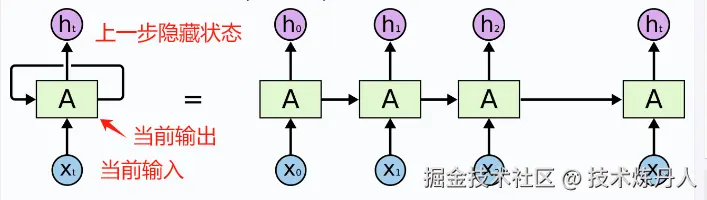
RNN核心在于循环连接 (Recurrent Connection),即网络的输出不仅取决于当前输入,还取决于之前所有时间步的输入,这种结构使得RNN能够处理任意长度的序列数据。
循环连接将上一步的隐藏状态传递到下一步,形成记忆。
- 每一步输入 = 当前数据 + 上一步的隐藏状态
- 每一步输出 = f(每一步输入)
举例: 就像人阅读句子时,理解当前单词会依赖前面读过的内容。(例如"他打开了__",你会预测"门"或"书")
RNN 工作机制
RNN在每个时间步执行以下计算:
- 接受当前输入 xt和前一时刻的隐藏状态 ht−1
- 计算新的隐藏状态 ht=f(Whh⋅ht−1+Wxh⋅xt+b)
- 产生输出 yt=g(Why⋅ht+c)
其中f和g通常是激活函数(如tanh或softmax)
python
import numpy as np
import random
import sys


class CharRNN:
    def __init__(self, data, hidden_size=100, seq_length=25, learning_rate=0.1):
        """
初始化字符级RNN模型
:param data: 训练文本数据
:param hidden_size: 隐藏层大小
:param seq_length: 序列长度
:param learning_rate: 学习率
"""
self.data = data
        self.hidden_size = hidden_size
        self.seq_length = seq_length
        self.learning_rate = learning_rate

        # 获取文本中所有唯一字符并创建映射
        self.chars = list(set(data))
        self.data_size = len(data)
        self.vocab_size = len(self.chars)

        # 存储字符:位置 映射关系
        self.char_to_idx = {ch: i for i, ch in enumerate(self.chars)}
        self.idx_to_char = {i: ch for i, ch in enumerate(self.chars)}

        # 初始化权重
        self.Wxh = np.random.randn(hidden_size, self.vocab_size) * 0.01  # 输入到隐藏层
        self.Whh = np.random.randn(hidden_size, hidden_size) * 0.01  # 隐藏层到隐藏层
        self.Why = np.random.randn(self.vocab_size, hidden_size) * 0.01  # 隐藏层到输出
        self.bh = np.zeros((hidden_size, 1))  # 隐藏层偏置
        self.by = np.zeros((self.vocab_size, 1))  # 输出层偏置

    def lossFun(self, inputs, targets, hprev):
        """
计算损失和梯度
:param inputs: 输入字符索引列表
:param targets: 目标字符索引列表
:param hprev: 上一时间步的隐藏状态
:return: 损失, 梯度, 最后一个时间步的隐藏状态
"""
# 存储中间值
        xs, hs, ys, ps = {}, {}, {}, {}
        hs[-1] = np.copy(hprev)
        loss = 0

        # 前向传播
        for t in range(len(inputs)):
            xs[t] = np.zeros((self.vocab_size, 1))  # 独热编码
            xs[t][inputs[t]] = 1
            hs[t] = np.tanh(np.dot(self.Wxh, xs[t]) + np.dot(self.Whh, hs[t - 1]) + self.bh)  # 隐藏状态
            ys[t] = np.dot(self.Why, hs[t]) + self.by  # 未归一化的输出
            ps[t] = np.exp(ys[t]) / np.sum(np.exp(ys[t]))  # 概率分布
            loss += -np.log(ps[t][targets[t], 0])  # 交叉熵损失

        # 反向传播计算梯度
        dWxh, dWhh, dWhy = np.zeros_like(self.Wxh), np.zeros_like(self.Whh), np.zeros_like(self.Why)
        dbh, dby = np.zeros_like(self.bh), np.zeros_like(self.by)
        dhnext = np.zeros_like(hs[0])

        for t in reversed(range(len(inputs))):
            dy = np.copy(ps[t])
            dy[targets[t]] -= 1  # 输出误差
            dWhy += np.dot(dy, hs[t].T)
            dby += dy

            dh = np.dot(self.Why.T, dy) + dhnext  # 隐藏层误差
            dhraw = (1 - hs[t] ** 2) * dh  # tanh导数
            dbh += dhraw
            dWxh += np.dot(dhraw, xs[t].T)
            dWhh += np.dot(dhraw, hs[t - 1].T)
            dhnext = np.dot(self.Whh.T, dhraw)

        # 梯度裁剪,防止梯度爆炸
        for dparam in [dWxh, dWhh, dWhy, dbh, dby]:
            np.clip(dparam, -5, 5, out=dparam)

        return loss, dWxh, dWhh, dWhy, dbh, dby, hs[len(inputs) - 1]

    def sample(self, h, seed_ix, n):
        """
从模型中采样生成字符序列
:param h: 初始隐藏状态
:param seed_ix: 初始字符索引
:param n: 生成的字符数量
:return: 生成的字符索引列表
"""
x = np.zeros((self.vocab_size, 1))
        x[seed_ix] = 1
        ixes = []

        for _ in range(n):
            h = np.tanh(np.dot(self.Wxh, x) + np.dot(self.Whh, h) + self.bh)
            y = np.dot(self.Why, h) + self.by
            p = np.exp(y) / np.sum(np.exp(y))
            ix = np.random.choice(range(self.vocab_size), p=p.ravel())
            x = np.zeros((self.vocab_size, 1))
            x[ix] = 1
            ixes.append(ix)

        return ixes

    def train(self, epochs=10):
        """
训练模型
:param epochs: 训练轮数
"""
# 准备训练数据
        n, p = 0, 0
        mWxh, mWhh, mWhy = np.zeros_like(self.Wxh), np.zeros_like(self.Whh), np.zeros_like(self.Why)
        mbh, mby = np.zeros_like(self.bh), np.zeros_like(self.by)  # 动量变量
        smooth_loss = -np.log(1.0 / self.vocab_size) * self.seq_length  # 初始损失

        for epoch in range(epochs):
            hprev = np.zeros((self.hidden_size, 1))  # 重置隐藏状态

            # 每次循环处理一个序列长度的数据
            while p + self.seq_length + 1 <= len(self.data):

                # inputs
                # 对应文本片段
                # data[0:3] = "abc",转换为索引后是[a的索引, b的索引, c的索引];

                inputs = [self.char_to_idx[ch] for ch in self.data[p:p + self.seq_length]]
                targets = [self.char_to_idx[ch] for ch in self.data[p + 1:p + self.seq_length + 1]]

                # 前向传播并计算梯度
                loss, dWxh, dWhh, dWhy, dbh, dby, hprev = self.lossFun(inputs, targets, hprev)
                smooth_loss = smooth_loss * 0.999 + loss * 0.001

                # 每100步打印一次损失
                if n % 100 == 0:
                    print(f'Epoch: {epoch}, Step: {n}, Loss: {smooth_loss:.4f}')

                    # 生成一个样本查看效果
                    sample_ix = self.sample(hprev, inputs[0], 200)
                    txt = ''.join(self.idx_to_char[ix] for ix in sample_ix)
                    print(f"Sample: {txt}\n")

                # 使用Adagrad更新权重
                for param, dparam, mem in zip(
                        [self.Wxh, self.Whh, self.Why, self.bh, self.by],
                        [dWxh, dWhh, dWhy, dbh, dby],
                        [mWxh, mWhh, mWhy, mbh, mby]
                ):
                    mem += dparam * dparam
                    param += -self.learning_rate * dparam / np.sqrt(mem + 1e-8)  # 加入小epsilon防止除零

                p += self.seq_length  # 移动到下一个序列
                n += 1

            p = 0  # 重置数据指针,开始新一轮训练


# 测试代码
if __name__ == "__main__":
    # 示例训练文本 - 可以替换为任何文本
    with open("test.txt", "w") as f:
        f.write("""Natural language processing (NLP) is a subfield of linguistics, computer science,
        and artificial intelligence concerned with the interactions between computers and human language.
        It focuses on how to program computers to process and analyze large amounts of natural language data.
        The goal is to enable computers to understand, interpret, and generate human language in a way that is useful.
        """)

    # 读取训练数据
    with open("test.txt", "r") as f:
        data = f.read()

    # 创建并训练RNN模型
    rnn = CharRNN(data, hidden_size=100, seq_length=25, learning_rate=0.1)
    print(f"训练数据长度: {len(data)} 字符")
    print(f"词汇表大小: {rnn.vocab_size} 个唯一字符")
    print("开始训练...")
    rnn.train(epochs=10)  # 训练10轮

    # 使用训练好的模型生成文本
    print("\n最终生成文本示例:")
    hprev = np.zeros((rnn.hidden_size, 1))
    start_char = random.choice(rnn.chars)  # 随机选择一个起始字符
    start_idx = rnn.char_to_idx[start_char]
    generated_indices = rnn.sample(hprev, start_idx, 500)  # 生成500个字符
    generated_text = ''.join(rnn.idx_to_char[ix] for ix in generated_indices)
    print(generated_text)
隐藏状态更新公式
隐藏状态是RNN的核心,用于记忆历史信息,其更新公式为:
ht=tanh(Wxh⋅xt+Whh⋅ht−1+bh)
- ht:当前时间步的隐藏状态(维度:隐藏层大小 × 1)
- xt:当前时间步的输入(字符的独热编码,维度:词汇表大小 × 1)
- ht−1:上一时间步的隐藏状态(维度:隐藏层大小 × 1)
- Wxh:输入到隐藏层的权重矩阵(维度:隐藏层大小 × 词汇表大小)
- Whh:隐藏层到自身的权重矩阵(维度:隐藏层大小 × 隐藏层大小)
- bh:隐藏层的偏置(维度:隐藏层大小 × 1)
- tanh(⋅):激活函数,将输出映射到-1, 1区间
输出层计算与概率分布
当前时间步的输出通过隐藏状态计算,并经softmax 归一化为概率分布
未归一化输出
yt=Why⋅ht+by
-
yt:未归一化的输出(维度:词汇表大小x1)
-
Why:隐藏层到输出层的权重矩阵(维度:词汇表大小 × 隐藏层大小)
-
by:输出层的偏置(维度:词汇表大小 × 1)
概率分布
pt(k)=∑i=1Vexp(yt(i))exp(yt(k))
-
pt(k):当前时间步输出字符为第$$$$个字符的概率
-
V:词汇表大小(唯一字符的数量)
损失函数 ( 交叉熵 损失)
L=−∑t=1Tlog(pt(y^t))
- T:序列长度(每个训练批次的字符数)
- y^t:第 t时间步的目标字符(真实标签)
- pt(y^t):模型预测目标字符 y^t的概率
这些公式构成了字符级RNN的核心逻辑:通过隐藏状态传递历史信息,基于当前输入和历史信息预测下一个字符,并通过损失函数优化模型参数 (Wxh,Whh,Why,bh,by)。
RNN 优缺点
优点:
- 能够处理边长序列
- 理论上可以记住任意长度的历史信息
- 参数共享(同一组权重参数用于所有时间步)
缺点:
-
串行计算(计算效率低,无法并行处理时间步) -
长依赖遗忘(梯度消失/爆炸问题,难以学习长期依赖)
长依赖解决:LSTM长短期记忆网络(Long Short-Term Memory)
LSTM:是一种特殊的递归神经网络,RNN改进的一种架构,专门设计用来解决标准RNN长期依赖问题
核心结构
LSTM引入了三个门控机制和一个记忆单元
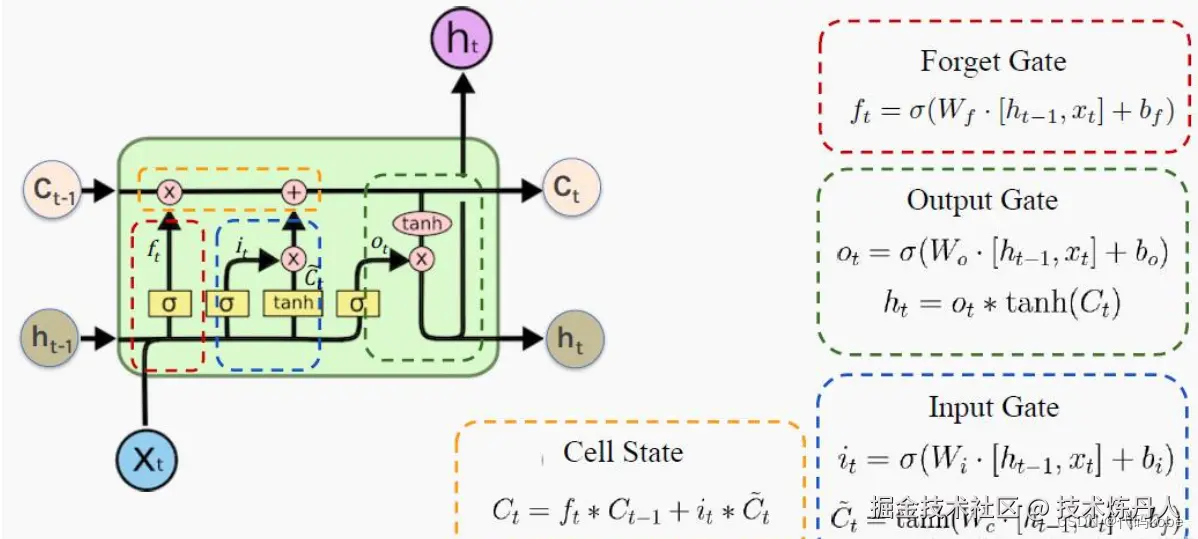
Ct: 细胞状态(记忆状态)
Xt: 输入信息
ht−1: 隐藏状态(基于 Ct得到的)
| 组件 | 功能 |
|---|---|
| 输入门 | 控制新信息的流入 |
| 遗忘门 | 决定丢弃哪些旧信息 |
| 输出门 | 控制输出的信息量 |
| 记忆单元 | 保存长期状态 |
实战
ini
class LSTMCell:
    def __init__(self, input_size, hidden_size):
        # 组合所有们的权重
        # 4个门(每个门输出维度为hidden_size),
        # input_size + hidden_size对应输入维度(当前输入x的维度input_size + 前一时刻隐藏状态h_prev的维度hidden_size)
        self.w = np.random.randn(4*hidden_size,input_size+hidden_size)
        self.b = np.random.randn(4*hidden_size,1)
        #保存方便分割
        self.hidden_size = hidden_size

    def forward(self, x,h_prev, c_prev):
        combined = np.vstack((h_prev,x))
        gates = np.dot(self.w, combined) + self.b

        hidden_size = self.hidden_size
        # 分割得到4个门
        f_gate = sigmoid(gates[:hidden_size])# 遗忘门
        i_gate = sigmoid(gates[hidden_size:2*hidden_size])# 输入门
        o_gate = sigmoid(gates[2*hidden_size:3*hidden_size])# 输出门
        c_candidate = sigmoid(gates[3*hidden_size:]) # 候选记忆

        #更新状态和隐藏状态
        c_next = f_gate* c_prev + i_gate * c_candidate
        h_next = o_gate * np.tanh(c_next)

        return h_next, c_next
前向传播过程实现了LSTM单元的核心计算,分为以下步骤:
步骤1:拼接输入
将前一时刻的隐藏状态h_prev和当前输入x垂直拼接,形成统一的输入向量:
ini
combined = np.vstack((h_prev, x)) # 形状为 (input_size + hidden_size, 1)公式:
combined=hprevx
(其中h_{\text{prev}为前一时刻隐藏状态, x为当前输入)
步骤2:计算所有门的线性组合
通过权重矩阵W和偏置b,一次性计算4个门的线性输出:
ini
gates = np.dot(self.W, combined) + self.b # 形状为 (4*hidden_size, 1)公式:
gates=W⋅combined+b
(其中 W为权重矩阵, b为偏置向量)
步骤3:分割并激活各个门
将gates分割为4个部分,分别通过激活函数得到4个门的输出:
-
遗忘门(f_gate) :控制前一时刻细胞状态
c_prev的保留比例(输出范围0~1,用sigmoid激活):inif_gate = sigmoid(gates[:hidden_size]) -
输入门(i_gate) :控制候选记忆细胞
c_candidate的加入比例(输出范围0~1,用sigmoid激活):inii_gate = sigmoid(gates[hidden_size:2*hidden_size]) -
输出门(o_gate) :控制当前细胞状态
c_next对隐藏状态h_next的贡献比例(输出范围0~1,用sigmoid激活):inio_gate = sigmoid(gates[2*hidden_size:3*hidden_size]) -
候选记忆细胞(c_candidate) :生成待加入细胞状态的新信息(输出范围-1~1,用tanh激活):
inic_candidate = np.tanh(gates[3*hidden_size:])
步骤4:更新细胞状态(长期记忆)
细胞状态c_next由两部分组成:前一时刻细胞状态经遗忘门筛选后的信息,加上输入门筛选后的候选记忆信息:
ini
c_next = f_gate * c_prev + i_gate * c_candidate公式:
cnext=f⊙cprev+i⊙c~
( \odo表示元素级乘法,c_{\text{prev}为前一时刻细胞状态)
步骤5:计算当前隐藏状态(短期记忆)
隐藏状态h_next由输出门控制,仅允许细胞状态的部分信息输出(细胞状态先经tanh压缩到-1~1,再与输出门相乘):
ini
h_next = o_gate * np.tanh(c_next)公式:
hnext=o⊙tanh(cnext)
核心公式总结
-
输入拼接: combined =hprevx
-
门控线性组合: gates=W⋅combined+b
-
遗忘门: f=σ(Wf⋅combined+bf
-
输入门: i=σ(Wi⋅combined+bi
-
输出门: o=σ(Wo⋅combined+bo
-
候选记忆: c~=tanh(Wc~⋅combined+bc~
-
细胞状态更新: cnext=f⊙cprev+i⊙c~
-
隐藏状态更新: hnext=o⊙tanh(cnext
LSTM 如何解决长期依赖问题
-
选择性记忆:遗忘门可以决定保留或丢弃特定信息
-
梯度通路:记忆单元提供了相对直接的梯度传播路径
-
信息保护:记忆内容不会被每个时间步的操作直接修改
推荐参考:blog.csdn.net/mary19831/a...
注意力机制(Attention Mechanism)
一种深度学习的重要技术,它模仿了人类视觉和认知过程中的注意力分配方式。就像你在阅读时会不自觉地将注意力集中在关键词上一样,注意力机制让神经网络能够动态地关注输入数据中最相关的部分。
基本概念
核心思想: 根据输入的不同部分当当前任务的重要性,动态分配不同的权重,这种权重不是固定的,而是根据上下文动态计算的。
数学表达
Attention(Q, K, V) = softmax(QK^T/√d_k)V
其中:
- Q (Query):当前需要计算输出的查询项
- K (Key):用于与查询项匹配的键
- V (Value):与键对应的实际值
- d_k:键的维度,用于缩放点积结果
为什么需要注意力机制
-
解决长距离依赖问题:传统RNN难以捕捉远距离词语间的关系
-
并行计算 能力:相比RNN的顺序处理,注意力可以并行计算
-
可解释性:注意力权重可以直观展示模型关注的重点
自注意力机制(Self Attention)
自注意力是注意力机制的一种特殊形式,它允许输入序列中的每个元素都与序列中的所有元素建立联系。
工作原理
-
对输入序列中的每个元素,计算其与所有元素的相似度得分
-
使用softmax函数将这些得分转化为权重(0-1之间)
-
用这些权重对对应的值进行加权求和,得到输出
ini
# 在自注意力中,query、key的形状通常为 (batch_size, seq_len, d_k),其中:
# batch_size:批次大小(如一次处理 2 个句子);
# seq_len:序列长度(如句子包含 3 个词);
# d_k:每个元素的特征维度(如每个词用 4 维向量表示)。

def self_attention(query,key,value):
    # 矩阵乘法要求:query与key的矩阵乘法需要满足query的最后一个维度 = key的倒数第二个维度。
    # query.size(-1)作用:获取query张量最后一个维度的大小(即d_k,特征维度),用于缩放注意力分数。

    scores = torch.matmul(query,key.transpose(-2,-1))/ (query.size(-1) **0.5)
    weights = F.softmax(scores,dim=-1)
    return torch.matmul(weights,value)
自注意力的优势
- 全局上下文感知:每个位置都能直接访问序列中所有位置的信息
- 位置无关性:不依赖序列顺序,适合处理各种结构化数据
- 高效计算:相比RNN的O(n)复杂度,自注意力可以并行计算
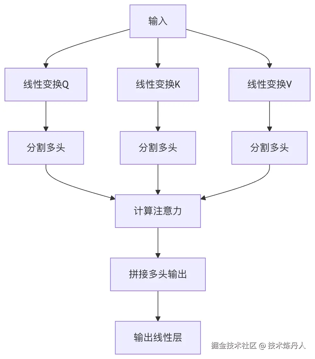
多头注意力机制(Multi-Head Attention)
多头注意力机制:是自注意力的扩展,它将注意力机制并行执行多次,然后将结果拼接起来。
结构组成
- 多个注意力头:通常使用8个或更多并行的注意力头
- 线性变换层:每个头有自己的Q、K、V变换矩阵
- 拼接和输出:将各头的输出拼接后通过线性层
实现示例
ini
# 多头注意力实现示例
class MultiHeadAttention(nn.Module):
    def __init__(self, d_model, num_heads):
        super().__init__()
        self.d_model = d_model
        self.num_heads = num_heads
        self.d_k = d_model // num_heads

        self.W_q = nn.Linear(d_model, d_model)
        self.W_k = nn.Linear(d_model, d_model)
        self.W_v = nn.Linear(d_model, d_model)
        self.W_o = nn.Linear(d_model, d_model)

    def forward(self, query, key, value):
        batch_size = query.size(0)

        # 线性变换并分割多头
        Q = self.W_q(query).view(batch_size, -1, self.num_heads, self.d_k)
        K = self.W_k(key).view(batch_size, -1, self.num_heads, self.d_k)
        V = self.W_v(value).view(batch_size, -1, self.num_heads, self.d_k)

        # 计算注意力
        scores = torch.matmul(Q, K.transpose(-2, -1)) / (self.d_k ** 0.5)
        weights = F.softmax(scores, dim=-1)
        output = torch.matmul(weights, V)

        # 拼接多头并输出
        output = output.transpose(1, 2).contiguous().view(batch_size, -1, self.d_model)
        return self.W_o(output)
多头注意力的优势
-
捕捉不同关系:每个头可以学习关注不同方面的关系
-
增强表达能力:比单头有更强的特征提取能力
-
稳定训练:多个头的组合可以减少模型对特定模式的依赖
Bert中的注意力
Bert(Bidirictional Encoder Representations from Transformers)
- 双向自注意力:同时考虑左右上下文
- 12/24层Transformer:堆叠多头注意力层
- 预训练任务:通过掩码语言模型和下一句预测任务学习通用表示
ini
# 使用HuggingFace Transformers库调用BERT
from transformers import BertModel, BertTokenizer

tokenizer = BertTokenizer.from_pretrained('bert-base-uncased')
model = BertModel.from_pretrained('bert-base-uncased')

inputs = tokenizer("Hello, my dog is cute", return_tensors="pt")
outputs = model(**inputs)

# 获取注意力权重
attention = outputs.attentions  # 包含各层的注意力权重
注意力机制的变体与扩展
1. 缩放点积注意力(Scaled Dot-Product Attention)
- 引入缩放因子(√d_k)防止softmax饱和
- 计算效率高,适合大规模应用
2. 加法注意力(Additive Attention)
- 使用单层前馈网络计算兼容性函数
- 适用于查询和键维度不同的情况
3. 局部注意力(Local Attention)
- 只关注输入的一个子集,降低计算复杂度
- 平衡了全局注意力和计算效率
4. 稀疏注意力(Sparse Attention)
- 只计算部分位置的注意力权重
- 如Longformer采用的滑动窗口注意力
基础注意力机制:
python
import torch
import torch.nn as nn
import torch.nn.functional as F

class SimpleAttention(nn.Module):
    def __init__(self, hidden_size):
        super(SimpleAttention, self).__init__()
        self.attention = nn.Linear(hidden_size, 1)

    def forward(self, encoder_outputs):
        # encoder_outputs: [batch_size, seq_len, hidden_size]
        attention_scores = self.attention(encoder_outputs).squeeze(2)  # [batch_size, seq_len]
        attention_weights = F.softmax(attention_scores, dim=1)
        context_vector = torch.bmm(attention_weights.unsqueeze(1), encoder_outputs)  # [batch_size, 1, hidden_size]
        return context_vector.squeeze(1), attention_weights