pytorch 学习笔记（2）-实现一个线性回归模型

搭建好python后对于内部的很多函数还是不太了解，按照下面的学习博客，理解内部具体的网络实现并代码实现一个线性回归模型并训练。

【从零开始学习深度学习】3. 基于pytorch手动实现一个线性回归模型并进行min--batch训练_pytorch mini batch-CSDN博客

网络模型：矩阵乘法-输入矩阵*权重 = 输出

损失函数：预测值与真实值的误差平方

优化函数：小批量随机梯度下降

pytorch中对梯度自动计算，存储tensor计算图，所以应该着重理解并注意是否梯度参与计算

python 复制代码

import numpy.random
import torch
from matplotlib import pyplot as plt
import numpy as np
from IPython import display
import random

import os
os.environ['KMP_DUPLICATE_LIB_OK'] = 'True'

num_inputs = 2
num_examples = 1000
w0 = [2,-3.4]
b0 = 4.2
data = torch.randn(num_examples, num_inputs,dtype=torch.float)
labels = w0[0] * data[:,0] + w0[1] * data[:,1] + b0
labels += torch.tensor(np.random.normal(0,0.01,size=labels.size())).float()

def data_iter(batch_size,data,labels):
    num_examples = data.shape[0]
    indices = list(range(num_examples)) #返回0-1000的序列
    random.shuffle(indices) #原地打乱indices列表的顺序
    for i in range(0,num_examples,batch_size):
        j = torch.LongTensor(indices[i:min(i+batch_size,num_examples)]) #返回indices打乱后从i-barch_size段的值，用作索引
        yield data.index_select(0,j), labels.index_select(0,j) #yield 惰性生成，每次只生成一组数据暂停，等第二次调用生成第二组

#将权重初始化成均值0，标准差0.01的正态随机数，偏差b初始化为0
w = torch.tensor(numpy.random.normal(0,0.01,(num_inputs,1)),dtype=torch.float)
b = torch.zeros(1).float()
#后续模型训练中,需要对这些参数求梯度来迭代参数的值，因此必须为true
w.requires_grad_(True)
b.requires_grad_(True)

#线性回归模型
def linreg(X, w, b):
    return torch.mm(X,w) + b #mm函数-矩阵乘法  输入*权重+偏差=输出 一个简单的线性回归网络模型

#损失函数
def squared_loss(y_hat,y):
    return (y_hat - y.view(y_hat.size()))**2/2  # 注意这里返回的是向量

#优化算法
def sgd(params, lr,batch_size):
    for param in params:
        param.data -= lr * param.grad / batch_size  #这里更改param时用的param.data，想要修改param的值，又不希望被autograd记录（不会影响反向传播），就对data操作

lr = 0.03
num_epochs = 3
batch_size = 10
net = linreg
loss = squared_loss

losses = []
for epoch in range(num_epochs):
    for X,y in data_iter(batch_size,data,labels):
        output = net(X,w,b)
        l = loss(output,y).sum()   # l是有关小批量X和y的损失
        l.backward() # 小批量的损失对模型参数求梯度
        sgd([w,b],lr,batch_size) # 使用小批量随机梯度下降迭代模型参数

        w.grad.data.zero_() #梯度清零
        b.grad.data.zero_()
    train_l = loss(net(data,w,b),labels) # 计算第一个迭代周期的损失
    losses.append(train_l.mean().item())
    print('echo %d,loss %f' % (epoch+1, train_l.mean().item()))

plt.plot(losses, label ="loss")
plt.xlabel('epoch')
plt.ylabel('loss')
plt.title('Training Loss')
plt.show()

print(f"True_W={ w0 },\n learn w ={ w.detach().numpy() }")   #detach()脱离计算图，numpy转到数组
print(f"True_b={ b0},\n learn b ={ b.detach().numpy() }")

输出

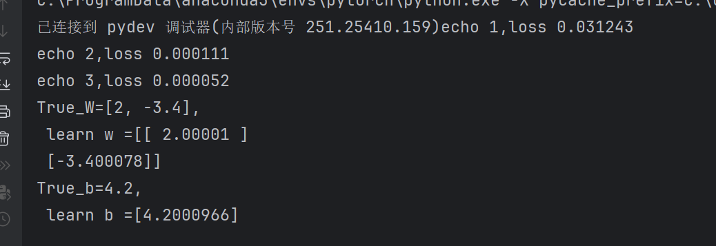
真实值和学习值很接近。