scanpy单细胞转录组python教程（四）：单样本数据分析之降维聚类及细胞注释

接上节（scanpy单细胞转录组python教程（一）：不同形式数据读取，scanpy单细胞转录组python教程（二）：单样本数据分析之数据质控，scanpy单细胞转录组python教程（三）：单样本数据分析之数据标准化、特征选择、细胞周期计算、回归等）。这一节是scanpy单细胞分析流程的最后一个内容了，完成降维聚类及细胞注释，这里我们还是推荐使用marker手动注释，自动注释这里先不演示。完成细胞注释，获得的结果是后续所有分析的基石。

首先加载数据：

复制代码

import pandas as pd
import scanpy as sc
sc.settings.verbosity = 3 
sc.settings.set_figure_params(dpi=80, facecolor="white")
adata = sc.read_h5ad('./adata.h5ad')
adata
# AnnData object with n_obs × n_vars = 8419 × 22022
# obs: 'n_genes', 'n_genes_by_counts', 'log1p_n_genes_by_counts', 'total_counts', 'log1p_total_counts', 'pct_counts_in_top_20_genes', 'pct_counts_mt', 'pct_counts_ribo', 'pct_counts_hb', 'S_score', 'G2M_score', 'phase'
# var: 'gene_ids', 'feature_types', 'n_cells', 'mt', 'ribo', 'hb', 'n_cells_by_counts', 'mean_counts', 'log1p_mean_counts', 'pct_dropout_by_counts', 'total_counts', 'log1p_total_counts', 'highly_variable', 'means', 'dispersions', 'dispersions_norm', 'mean', 'std'
# uns: 'hvg', 'log1p', 'pca', 'phase_colors'
# obsm: 'X_pca'
# varm: 'PCs'
# layers: 'counts', 'log1p_norm'

PCA降维：通过运行主成分分析（PCA）来降低数据的维度。运行结束后可以使用sc.pl.pca_variance_ratio函数展示PC，默认展示前30个PCs，来看看单个PC分量对数据总方差的贡献情况，这个类似于seurat中的Eblowplot。以便让我们在后续的分析中选择合适的PCs。PCs的选择实际中可能需要自行确定调整。

复制代码

sc.tl.pca(adata, svd_solver="arpack",use_highly_variable=True)
sc.pl.pca_variance_ratio(adata, log=False,n_pcs=50)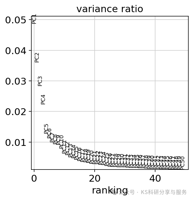

Clustering：使用scanpy函数sc.pp.neighbors细胞的邻域图。这里我们选择前20个主成分调用此函数，这些主成分能够捕捉到数据集中的大部分变异。

复制代码

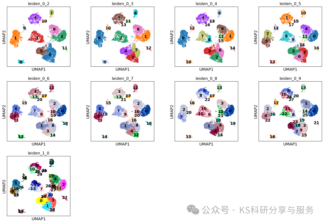
sc.pp.neighbors(adata, n_neighbors=10, n_pcs=20)

Clustering the neighborhood graph scanpy 中，默认的分辨率参数为1.0。但在许多情况下，我们可能希望尝试不同的分辨率参数来控制聚类的粗细程度。因此，可以将聚类结果保存在指定的key，用于指示所选的分辨率。通常可以多选择几个分辨率，类似于seurat，一般0.2-1.2就足够获取合适的结果。

复制代码

# sc.tl.leiden(
#   adata,
#   resolution=0.9,
#   random_state=0,
#   flavor="igraph",
#   n_iterations=2,
#   directed=False,)

#首次运行可以出现这个error，Please install the igraph package: `conda install -c conda-forge python-igraph` or `pip3 install igraph`.
#ImportError: Please install the leiden algorithm: `conda install -c conda-forge leidenalg` or `pip3 install leidenalg`.
#安装igraph即可： pip install igraph -i https://pypi.tuna.tsinghua.edu.cn/simple
#pip install leidenalg -i https://pypi.tuna.tsinghua.edu.cn/simple
list_leiden_res = [0.2, 0.3, 0.4, 0.5, 0.6, 0.7, 0.8, 0.9, 1.0]
for leiden_res in list_leiden_res:
            print(leiden_res)
            sc.tl.leiden(adata, resolution=leiden_res, key_added='leiden_'+str(leiden_res).replace(".", "_"))
            
            
# 0.2
# running Leiden clustering
# finished: found 12 clusters and added
# 'leiden_0_2', the cluster labels (adata.obs, categorical) (0:00:03)
# 0.3
# running Leiden clustering
# finished: found 14 clusters and added
# 'leiden_0_3', the cluster labels (adata.obs, categorical) (0:00:02)
# 0.4
# running Leiden clustering
# finished: found 17 clusters and added
# 'leiden_0_4', the cluster labels (adata.obs, categorical) (0:00:03)
# 0.5
# running Leiden clustering
# finished: found 18 clusters and added
# 'leiden_0_5', the cluster labels (adata.obs, categorical) (0:00:02)
# 0.6
# running Leiden clustering
# finished: found 21 clusters and added
# 'leiden_0_6', the cluster labels (adata.obs, categorical) (0:00:02)
# 0.7
# running Leiden clustering
# finished: found 22 clusters and added
# 'leiden_0_7', the cluster labels (adata.obs, categorical) (0:00:02)
# 0.8
# running Leiden clustering
# finished: found 23 clusters and added
# 'leiden_0_8', the cluster labels (adata.obs, categorical) (0:00:02)
# 0.9
# running Leiden clustering
# finished: found 28 clusters and added
# 'leiden_0_9', the cluster labels (adata.obs, categorical) (0:00:02)
# 1.0
# running Leiden clustering
# finished: found 30 clusters and added
# 'leiden_1_0', the cluster labels (adata.obs, categorical) (0:00:03)
list_leiden_res = [0.2, 0.3, 0.4, 0.5, 0.6, 0.7, 0.8, 0.9, 1.0]
resolutions = ['leiden_' + str(res).replace(".", "_") for res in list_leiden_res]
resolutions
#可视化所有分辨率下的结果
sc.pl.umap(
    adata,
    color= resolutions,
    legend_loc="on data",
)

Finding marker genes：鉴定marker基因，用于后续的分群注释。前面的res选择一个差不多合适的即可，对于大分群，也没必要一次性选择很大的res。

复制代码

sc.tl.rank_genes_groups(adata, groupby = "leiden_0_3", method="wilcoxon",layer='log1p_norm')
sc.pl.rank_genes_groups(adata, n_genes=25, sharey=False)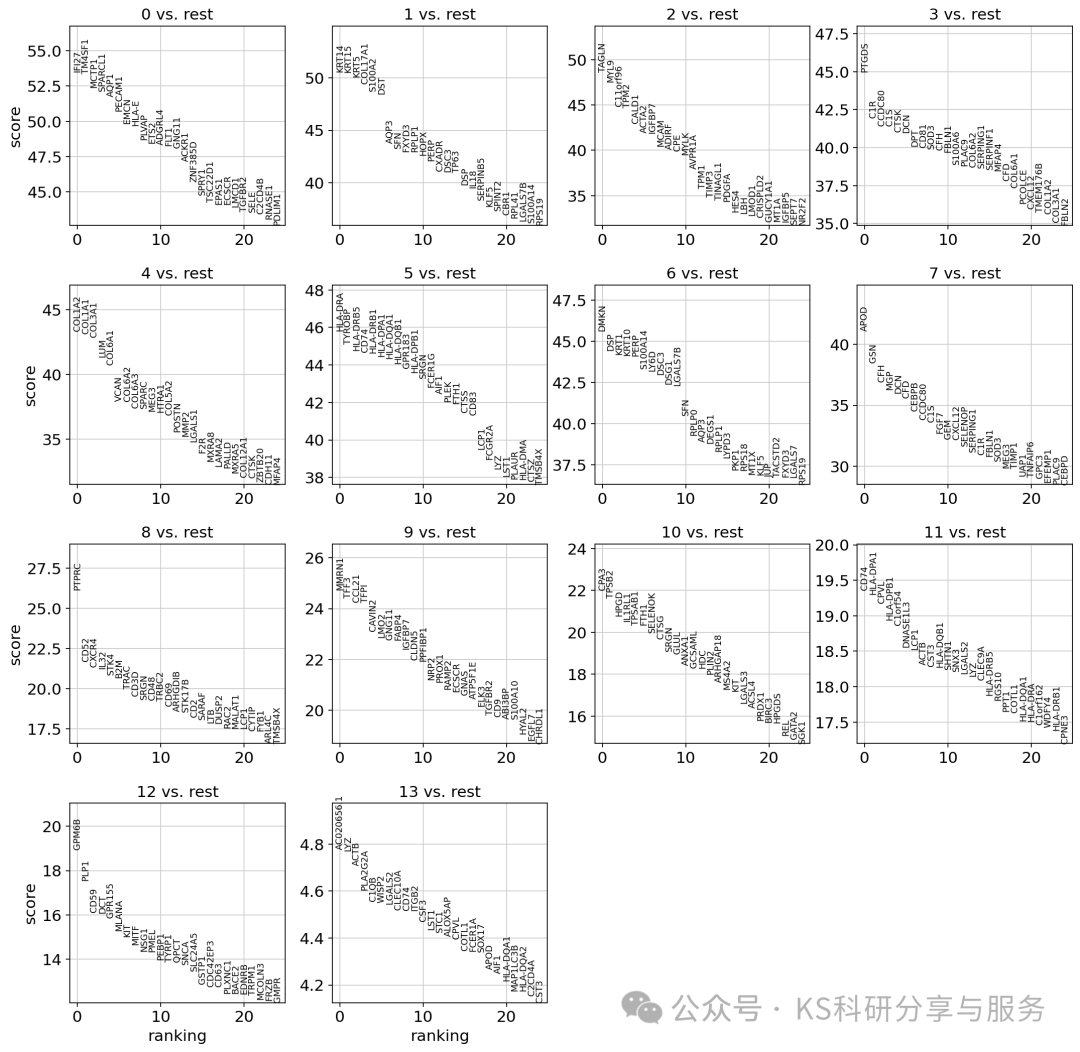

复制代码

# 将结果转换为 DataFrame.
marker_genes_df = sc.get.rank_genes_groups_df(adata, group=None, key='rank_genes_groups')
print(marker_genes_df.head())
#筛选显著性的结果
significant_markers = marker_genes_df[(marker_genes_df['pvals_adj'] < 0.05) & (marker_genes_df['logfoldchanges'] > 1)]
significant_markers

cell annotation：细胞的注释我还是倾向于手动注释，使用marker基因。使用经典的marker，dotplot看看cluster表达情况。

复制代码

marker_genes = [*["KRT5", "KRT10", "KRT14", "KRT15"], 
    *["THY1", "COL1A1", "COL11A1"], 
    *["CD3D", "CD8A", "CD4","IKZF2", "CCL5"], 
    *["CD14", "CD86", "CD163", "CD1A", "CLEC9A", "XCR1"], 
    *["MITF", "SOX10", "MLANA"], 
    *["VWF", "PECAM1", "SELE"], 
    *["FLT4", "LYVE1"],  
    *["TPM1", "TAGLN", "MYL9"], 
    *["TRPC6", "CCL19"], 
    *["KIT", "TPSB2", "HPGD"], 
    *["ITGB8", "CD200", "SOX9"]]
sc.pl.dotplot(adata, marker_genes, groupby="leiden_0_3",dendrogram=True);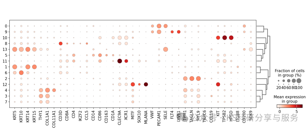

复制代码

#注释celltype
cellAnno = {
    "0": "Endothlial",
    "1": "Kers",
    "2": "MuCs",
    "3": "Fibs",
    "4": "Fibs",
    "5": "APCs",
    "6": "Kers",
    "7": "Fibs",
    "8": "Tcells",
    "9": "Lym",
    "10":"Mast",
    "11":"APCs",
    "12":"Mela",
    "13":"lowQ"}
#将上面的注释字典与adata中的leiden_0_3 match，并且形成新的一列obs celltype
adata.obs["celltype"] = adata.obs.leiden_0_3.map(cellAnno)
adata
# AnnData object with n_obs × n_vars = 8419 × 22022
# obs: 'n_genes', 'n_genes_by_counts', 'log1p_n_genes_by_counts', 'total_counts', 'log1p_total_counts', 'pct_counts_in_top_20_genes', 'pct_counts_mt', 'pct_counts_ribo', 'pct_counts_hb', 'S_score', 'G2M_score', 'phase', 'leiden_res0_3', 'leiden_res0_5', 'leiden_res1', 'leiden_0_2', 'leiden_0_3', 'leiden_0_4', 'leiden_0_5', 'leiden_0_6', 'leiden_0_7', 'leiden_0_8', 'leiden_0_9', 'leiden_1_0', 'celltype'
# var: 'gene_ids', 'feature_types', 'n_cells', 'mt', 'ribo', 'hb', 'n_cells_by_counts', 'mean_counts', 'log1p_mean_counts', 'pct_dropout_by_counts', 'total_counts', 'log1p_total_counts', 'highly_variable', 'means', 'dispersions', 'dispersions_norm', 'mean', 'std'
# uns: 'hvg', 'log1p', 'pca', 'phase_colors', 'neighbors', 'umap', 'leiden_res0_3', 'leiden_res0_5', 'leiden_res1', 'leiden_res0_3_colors', 'leiden_res0_5_colors', 'leiden_res1_colors', 'leiden_0_2', 'leiden_0_3', 'leiden_0_4', 'leiden_0_5', 'leiden_0_6', 'leiden_0_7', 'leiden_0_8', 'leiden_0_9', 'leiden_1_0', 'leiden_0_2_colors', 'leiden_0_3_colors', 'leiden_0_4_colors', 'leiden_0_5_colors', 'leiden_0_6_colors', 'leiden_0_7_colors', 'leiden_0_8_colors', 'leiden_0_9_colors', 'leiden_1_0_colors', 'rank_genes_groups', 'dendrogram_leiden_0_3'
# obsm: 'X_pca', 'X_umap'
# varm: 'PCs'
# layers: 'counts', 'log1p_norm'
# obsp: 'distances', 'connectivities'
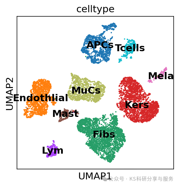
sc.pl.umap(adata, color=["celltype"])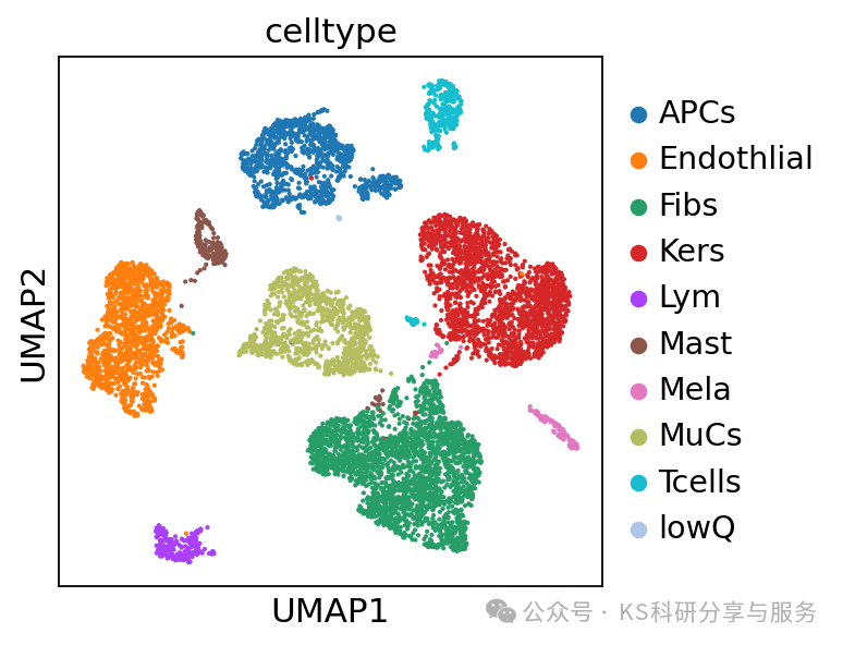

复制代码

#lowQ这群只有8个细胞，质量不好，所以我们决定将这群细胞删除，在删除前，将原来的数据备份
adata_all = adata.copy()
adata_filtered = adata[~adata.obs['celltype'].isin(['lowQ']), :].copy()
adata_filtered
sc.pl.umap(
    adata_filtered,
    color= 'celltype',
    legend_loc="on data",
)

删除细胞后，需要重新计算邻居图等依赖细胞数的结构，运行neighbors and umap！

sc.pp.neighbors(adata_filtered, n_neighbors=10, n_pcs=20)
sc.tl.umap(adata_filtered)
sc.pl.umap(
    adata_filtered,
    color= 'celltype',
    legend_loc="on data",
)