文章目录
-
- 回顾GPU的原理
- 基准测试
-
- benchmark
-
- 将`sleep`传入`benchmark`
- 将`矩阵乘法`传入`benchmark`
- 将`MLP`传入`benchmark`
-
- nvtx的作用
- [分别在step、layer数量、batch size、dimension上进行线性扩展](#分别在step、layer数量、batch size、dimension上进行线性扩展)
- 性能分析-profiler
- 内核融合的思想
- 不同版本的GELU实现方式
- Triton
-
- [Triton vs Cuda](#Triton vs Cuda)
- triton的gelu实现
- PTX
- 不同版本的gelu对比
- 不同版本的softmax
课程内容:
- 介绍基准测试和性能分析的基础知识
- 展示用C++编写cuda内核
- 介绍triton框架的使用
回顾GPU的原理
GPU的结构
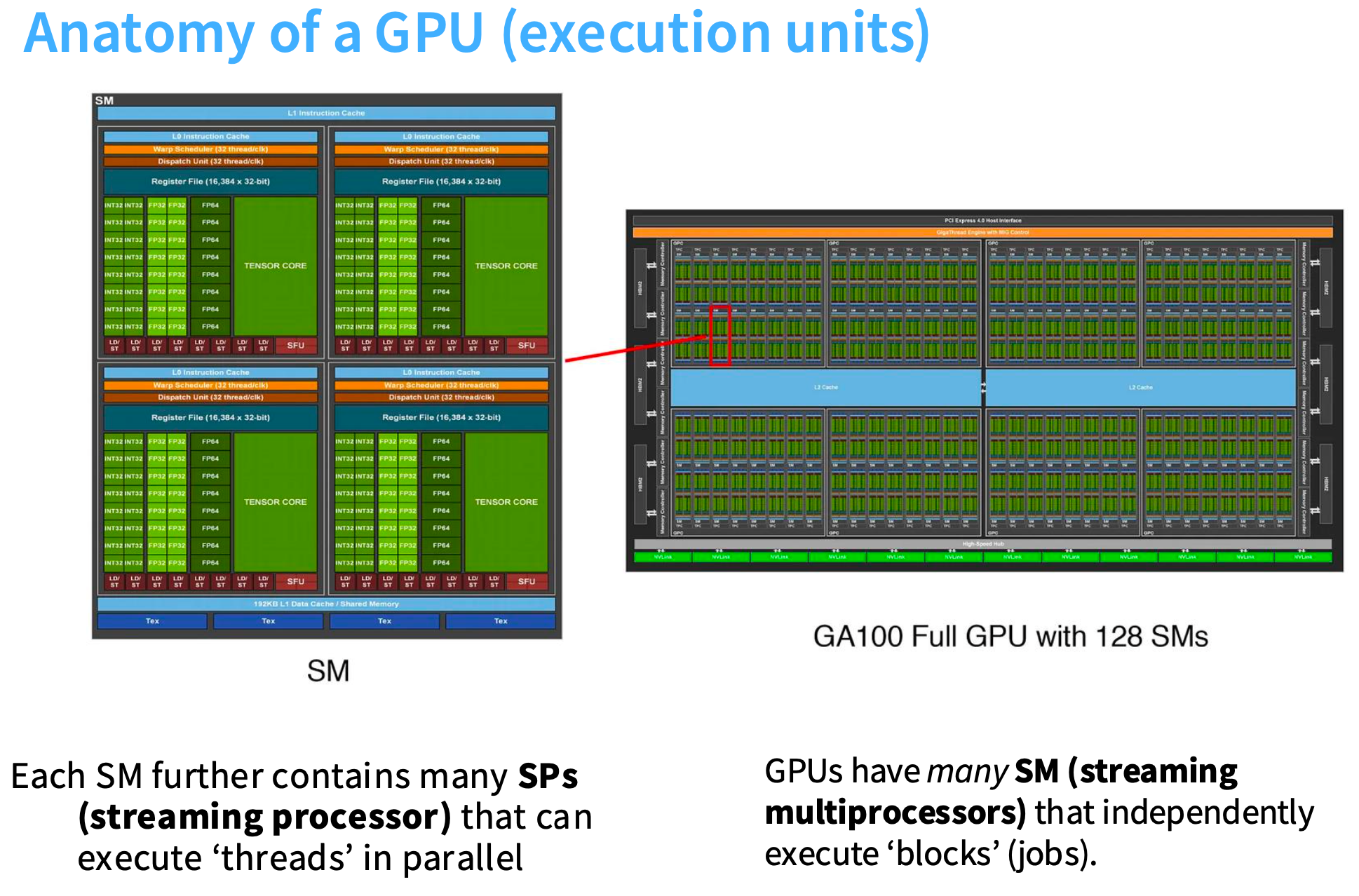
当我们拥有A100或H100这类设备时, 会有大量SM流式多处理器, 每个SM内部包含大量计算单元, 我们有FP32或FP64精度的计算单元,每个SM将启动大量线程。
我们还有内存层次结构, 其中DRAM或全局内存容量大但速度慢, 然后是更快的缓存层。
- DRAM A100: 80GB - big, slow
- L2 cache A100: 40MB
- L1 cache A100: 192KB per SM - small, fast
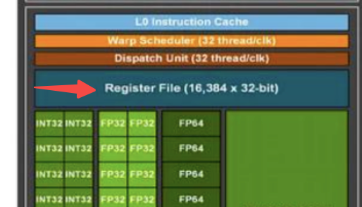
有一个叫寄存器文件的组件, 运行非常快, 是每个线程可访问的内存,在编写GPU高性能代码时会大量使用这些寄存器。
执行模型的基本结构
- 有一组线程块, 每个块会被调度到单个SM上执行。
- 尤其是在使用Triton等框架编写代码时, 每个块内包含大量线程, 这些线程实际执行计算任务。
- 如果你有一个向量, 你需要对向量元素进行操作, 你会编写代码让每个线程介入, 可能同时处理向量的几个元素, 所有线程共同完成向量处理
Q:什么是线程块?
A:线程块是同时执行的线程组(wrap)。线程块存在的原因是减少控制单元需求, 因为同时执行所有线程, 在同一时间, 无需为每个线程单独控制, 只需要控制线程块组。
例如, GPU更注重计算与简化控制,所以计算单元比线程调度器多得多, 能高效并行处理无需控制。而CPU会有更多硅面积用于控制和分支预测这类功能。
Q:为什么需要线程块这种结构呢, 为什么不直接使用全局线程?A:
- 线程块之间可以互相通信, 共享内存资源,在SM内部速度极快。
- 当你需要进行矩阵乘法时, 需要在不同线程间传递信息,在线程块内这种通信非常高效。
- 跨线程块或组的通信成本很高, 需要尽量将数据保留在同一线程块内, 或同一组别中, 这样能保持极高的运行速度, 这速度堪比L1缓存,
- 无法进行跨块同步, 因为你无法控制会发生什么
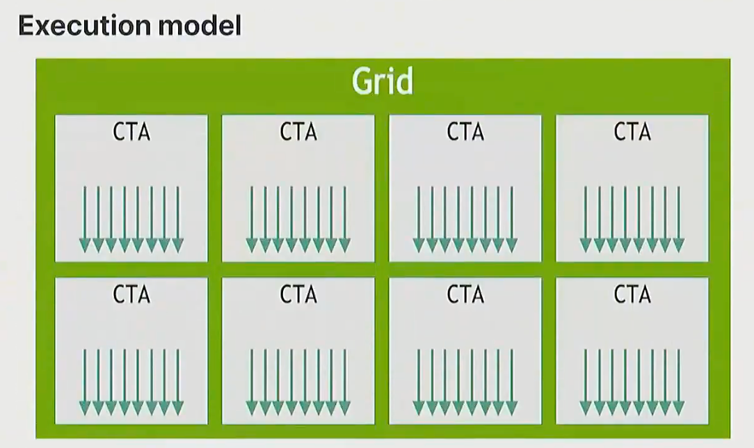
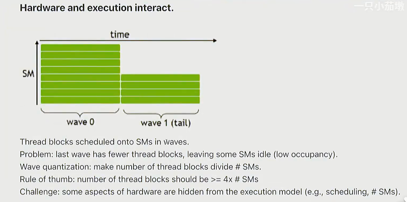
wave
线程被分组为连续的几个线程快,这就是一个波, 它们会几乎同时执行。
Q:如何确保所有波的计算量均衡?
A:调整线程块数量, 理想情况下应匹配SM数量, 并确保每个波的工作量均衡。因此我们理想情况下应有更多线程块, 并尽量实现高性能代码
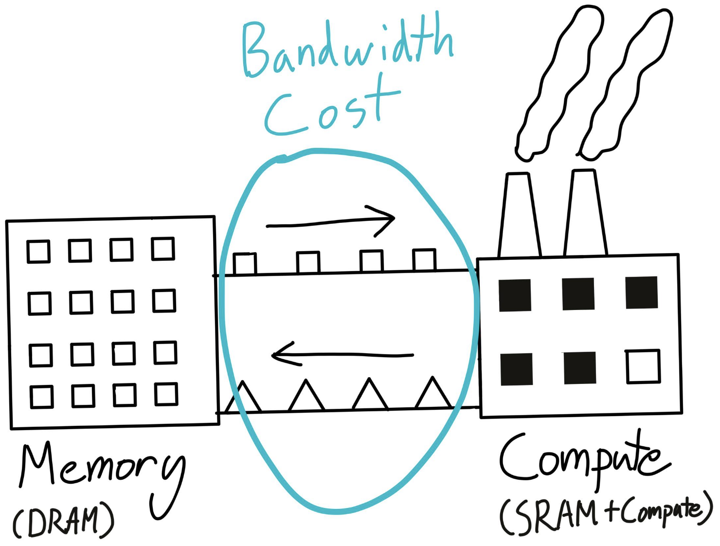
算术强度(Arithmetic Intensity: # FLOPS/ # bytes)
目标是,保持算术强度高。
即,希望浮点运算更多, 而非内存移动字节数,
因为计算扩展速度远快于内存扩展, 因此大部分时间计算会受限于内存。
基准测试
benchmark
两个重要操作:
-- warmup :第一次执行时有很多初始化操作,使用warmup后,可以确保不测量启动速度,而是稳定状态的速度
-- torch.cuda.synchronize:确保GPU和CPU状态同步, 没有排队的任务在运行, 处于代码执行的同一阶段, 在代码执行进度上一致。
原因:
- CPU和GPU是计算机中的独立计算单元, 它们可以独立运行。执行模型的代码运行在CPU上,运行时会分发大量CUDA内核到GPU,GPU开始执行。而CPU会继续运行,不会等待GPU执行完成。
- 这对高性能代码很友好, 但基准测试时会立即发现问题。
- 如果你在做基准测试, 模型在GPU后台运行, CPU在做其他事情, 实际上没有测量GPU执行时间。
python
# https://github.com/stanford-cs336/spring2025-lectures/blob/main/lecture_06.py
def benchmark(description: str, run: Callable, num_warmups: int = 1, num_trials: int = 3):
    """Benchmark `func` by running it `num_trials`, and return all the times."""
    # Warmup: first times might be slower due to compilation, things not cached.
    # Since we will run the kernel multiple times, the timing that matters is steady state.
    for _ in range(num_warmups):
        run()
    if torch.cuda.is_available():
        torch.cuda.synchronize()  # Wait for CUDA threads to finish (important!)

    # Time it for real now!
    times: list[float] = [] # @inspect times, @inspect description
    for trial in range(num_trials):  # Do it multiple times to capture variance
        start_time = time.time()

        run()  # Actually perform computation
        if torch.cuda.is_available():
            torch.cuda.synchronize()  # Wait for CUDA threads to finish (important!)

        end_time = time.time()
        times.append((end_time - start_time) * 1000) # @inspect times

    mean_time = mean(times) # @inspect mean_time
return mean_time将sleep传入benchmark
python
benchmark("sleep", lambda : time.sleep(50 / 1000))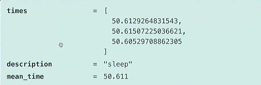
将矩阵乘法传入benchmark
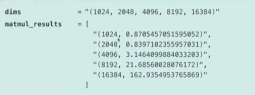
python
if torch.cuda.is_available():
     dims = (1024, 2048, 4096, 8192, 16384)  # @inspect dims
 else:
     dims = (1024, 2048)  # @inspect dims

 matmul_results = []
 for dim in dims:
     # @ inspect dim
     result = benchmark(f"matmul(dim={dim})", run_operation2(dim=dim, operation=lambda a, b: a @ b))
     matmul_results.append((dim, result))  # @inspect matmul_results
结论:
- 随着矩阵尺寸的增大,运行时间呈现超线性扩展。
- 在小尺寸时,时间完全没有增长。因为进行矩阵乘法存在固定开销, 这些数字需要从CPU传输到GPU。启动内核等操作也有开销, 因此并非完全超线性, 直到接近零点。但一旦矩阵足够大, 我们看到预期的扩展效果, 与我们的矩阵乘法一致。
将MLP传入benchmark
python
# https://github.com/stanford-cs336/spring2025-lectures/blob/main/lecture_06_mlp.py
import torch
import torch.nn as nn
import torch.cuda.nvtx as nvtx

def get_device(index: int = 0) -> torch.device:
    """Try to use the GPU if possible, otherwise, use CPU."""
    if torch.cuda.is_available():
        return torch.device(f"cuda:{index}")
    else:
        return torch.device("cpu")

class MLP(nn.Module):
    """Simple MLP: linear -> GeLU -> linear -> GeLU -> ... -> linear -> GeLU"""
    def __init__(self, dim: int, num_layers: int):
        super().__init__()
        self.layers = nn.ModuleList([nn.Linear(dim, dim) for _ in range(num_layers)])

    def forward(self, x: torch.Tensor):
        # Mark the entire forward pass
        for i, layer in enumerate(self.layers):
            # Mark each layer's computation separately
            with nvtx.range(f"layer_{i}"):
                x = layer(x)
                x = torch.nn.functional.gelu(x)

        return x

def run_mlp(dim: int, num_layers: int, batch_size: int, num_steps: int, use_optimizer: bool = False):
    """Run forward and backward passes through an MLP.

    Args:
        dim: Dimension of each layer
        num_layers: Number of linear+GeLU layers
        batch_size: Number of samples to process at once
        num_steps: Number of forward/backward iterations
        use_optimizer: Whether to use Adam optimizer for weight updates
    """
    # Define a model (with random weights)
    with nvtx.range("define_model"):
        model = MLP(dim, num_layers).to(get_device())

    # Initialize optimizer if requested
    optimizer = torch.optim.Adam(model.parameters()) if use_optimizer else None

    # Define an input (random)
    with nvtx.range("define_input"):
        x = torch.randn(batch_size, dim, device=get_device())

    # Run the model `num_steps` times
    for step in range(num_steps):
        if step > 10:
            # start profiling after 10 warmup iterations
            torch.cuda.cudart().cudaProfilerStart()

        nvtx.range_push(f"step_{step}")

        # Zero gradients
        if use_optimizer:
            optimizer.zero_grad()
        else:
            model.zero_grad(set_to_none=True)

        # Forward
        with nvtx.range("forward"):
            y = model(x).mean()

        # Backward
        with nvtx.range("backward"):
            y.backward()

        # Optimizer step if enabled
        if use_optimizer:
            with nvtx.range("optimizer_step"):
                #print(f"Step {step}, loss: {y.item():.6f}")
                optimizer.step()

        nvtx.range_pop()

def main():
    # Run a larger model if GPU is available
    if torch.cuda.is_available():
        print("Running on GPU")
        run_mlp(dim=4096, num_layers=64, batch_size=1024, num_steps=15, use_optimizer=True)
    else:
        print("Running on CPU")
        run_mlp(dim=128, num_layers=16, batch_size=128, num_steps=15, use_optimizer=True)

if __name__ == "__main__":
    main()
nvtx的作用
代码中的nvtx是NVIDIA提供的NVTX(NVIDIA Tools Extension)库的接口,主要用于在代码中插入标记(markers)或范围(ranges),以便在NVIDIA的性能分析工具(如Nsight Systems、Nsight Compute等)中可视化和分析程序的执行流程与时间分布。
- 标记关键操作阶段:
- 使用
nvtx.range("define_model")标记模型定义阶段 - 使用
nvtx.range("define_input")标记输入数据定义阶段 - 用
nvtx.range("forward")和nvtx.range("backward")分别标记前向传播和反向传播阶段
- 划分迭代步骤:
- 通过
nvtx.range_push(f"step_{step}")和nvtx.range_pop()标记每个迭代步骤的开始和结束
- 性能分析辅助:
- 这些标记会被NVIDIA的性能分析工具捕获,生成时间线可视化
- 帮助开发者识别程序中的性能瓶颈,如哪部分操作耗时最长
- 便于分析不同阶段(如前向/反向传播)的时间占比,优化代码效率
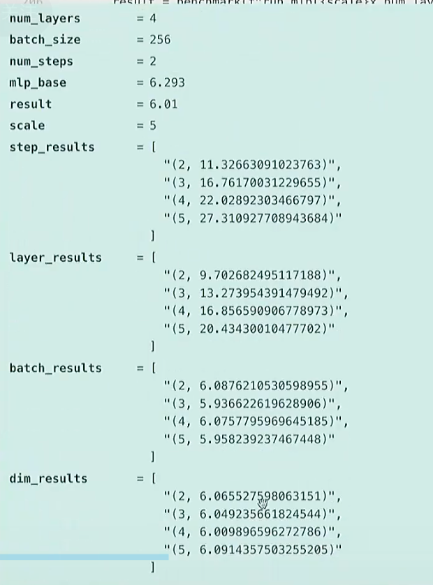
分别在step、layer数量、batch size、dimension上进行线性扩展
python
dim = 256  # @inspect dim
num_layers = 4  # @inspect num_layers
batch_size = 256  # @inspect batch_size
num_steps = 2  # @inspect num_steps

mlp_base = benchmark("run_mlp", run_mlp(dim=dim, num_layers=num_layers, batch_size=batch_size, num_steps=num_steps)) # @inspect mlp_base


text("Scale the number of steps.")
step_results = []
for scale in (2, 3, 4, 5):
    result = benchmark(f"run_mlp({scale}x num_steps)",
                     run_mlp(dim=dim, num_layers=num_layers,
                            batch_size=batch_size, num_steps=scale * num_steps)) # @inspect result, @inspect scale, @inspect num_steps
    step_results.append((scale, result))  # @inspect step_results

text("Scale the number of layers.")
layer_results = []
for scale in (2, 3, 4, 5):
    result = benchmark(f"run_mlp({scale}x num_layers)",
                     run_mlp(dim=dim, num_layers=scale * num_layers,
                            batch_size=batch_size, num_steps=num_steps)) # @inspect result, @inspect scale, @inspect num_layers, @inspect num_steps
    layer_results.append((scale, result))  # @inspect layer_results

text("Scale the batch size.")
batch_results = []
for scale in (2, 3, 4, 5):
    result = benchmark(f"run_mlp({scale}x batch_size)",
                     run_mlp(dim=dim, num_layers=num_layers,
                            batch_size=scale * batch_size, num_steps=num_steps)) # @inspect result, @inspect scale, @inspect num_layers, @inspect num_steps
    batch_results.append((scale, result))  # @inspect batch_results

text("Scale the dimension.")
dim_results = []
for scale in (2, 3, 4, 5):
    result = benchmark(f"run_mlp({scale}x dim)",
                     run_mlp(dim=scale * dim, num_layers=num_layers,
                            batch_size=batch_size, num_steps=num_steps)) # @inspect result, @inspect scale, @inspect num_layers, @inspect num_steps
    dim_results.append((scale, result))  # @inspect dim_results
结论 : step和层数大小,与时间呈线性关系
性能分析-profiler
教程地址:https://docs.pytorch.org/tutorials/recipes/recipes/profiler_recipe.html
python
def profile(description: str, run: Callable, num_warmups: int = 1, with_stack: bool = False):
    # Warmup
    for _ in range(num_warmups):
        run()
    if torch.cuda.is_available():
        torch.cuda.synchronize()  # Wait for CUDA threads to finish (important!)

    # Run the code with the profiler
    with torch.profiler.profile(
            activities=[ProfilerActivity.CPU, ProfilerActivity.CUDA],
            # Output stack trace for visualization
            with_stack=with_stack,
            # Needed to export stack trace for visualization
            experimental_config=torch._C._profiler._ExperimentalConfig(verbose=True)) as prof:
        run()
        if torch.cuda.is_available():
            torch.cuda.synchronize()  # Wait for CUDA threads to finish (important!)

    # Print out table
    table = prof.key_averages().table(sort_by="cuda_time_total",
                                      max_name_column_width=80,
                                      row_limit=10)
    #text(f"## {description}")
    #text(table, verbatim=True)

    # Write stack trace visualization
    if with_stack:
        text_path = f"var/stacks_{description}.txt"
        svg_path = f"var/stacks_{description}.svg"
        prof.export_stacks(text_path, "self_cuda_time_total")

    return table
add
matmul
matmul(dim=128)
cdist
gelu
softmax
python
def pytorch_softmax(x: torch.Tensor):
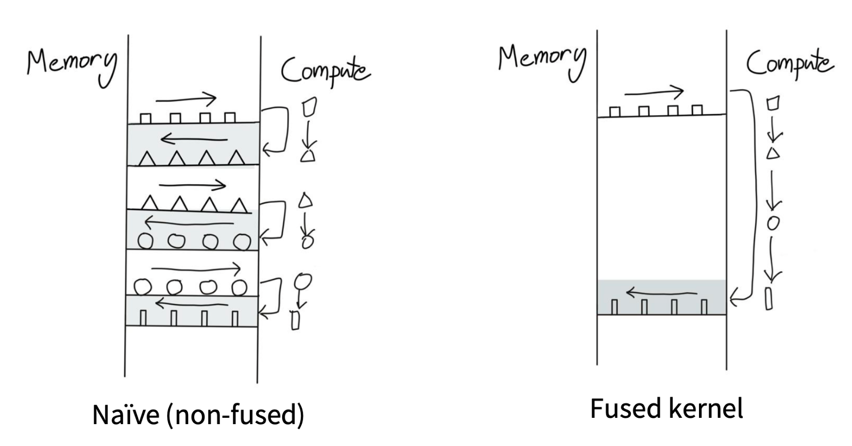
return torch.nn.functional.softmax(x, dim=-1)内核融合的思想
可以参考【cs336学习笔记】第5课详解GPU架构,性能优化
不同版本的GELU实现方式
1.pytorch版 vs 手动实现版
pytorch官方实现:https://docs.pytorch.org/docs/stable/generated/torch.nn.GELU.html
python
def pytorch_gelu(x: torch.Tensor):
    # Use the tanh approximation to match our implementation
    return torch.nn.functional.gelu(x, approximate="tanh")
python
def manual_gelu(x: torch.Tensor):
    return 0.5 * x * (1 + torch.tanh(0.79788456 * (x + 0.044715 * x * x * x)))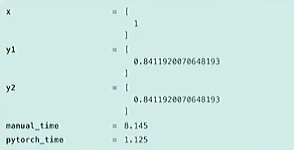
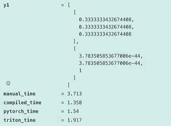
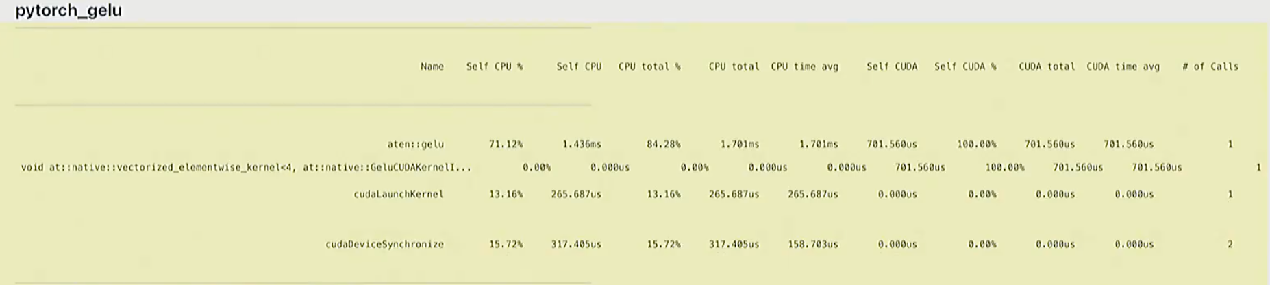
结论:
-
y1和y2的值相等,但是运行时间上差了8倍
-
manual_gelu是很朴素的思想,一步一步操作,有大量算子参与运算,例如
BinaryFunctor<f...调用了三次cuda kernel
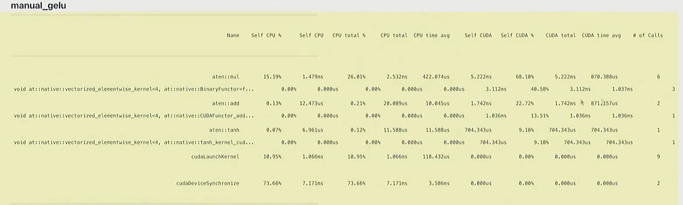
-
pytorch是算子融合后的版本,只调用了一次cuda kernel
2. cuda实现GELU
step1. C++实现的gelu函数,文件名:gelu.cu
c
#include <math.h>               // 包含标准数学函数(如tanh)
#include <torch/extension.h>    // PyTorch扩展开发必备头文件,提供张量操作等接口
#include <c10/cuda/CUDAException.h>  // CUDA错误处理工具

/**
 * CUDA核函数:计算GELU激活函数
 * 每个线程处理输入张量中的一个元素
 *
 * @param in 输入张量的数据指针(GPU内存)
 * @param out 输出张量的数据指针(GPU内存)
 * @param num_elements 张量中元素的总数量
 */
__global__ void gelu_kernel(float* in, float* out, int num_elements) {
    // 计算当前线程负责处理的元素索引
    // blockIdx.x: 当前线程块在网格中的索引
    // blockDim.x: 每个线程块中包含的线程数
    // threadIdx.x: 当前线程在线程块中的索引
    int i = blockIdx.x * blockDim.x + threadIdx.x;

    // 边界检查:确保线程只处理有效范围内的元素
    // 当总元素数不是线程块大小的整数倍时,避免越界访问
    if (i < num_elements) {
        // GELU激活函数计算公式(近似实现)
        // 原始公式:GELU(x) = 0.5 * x * (1 + erf(x / sqrt(2)))
        // 这里使用等价近似:0.5 * x * (1 + tanh(sqrt(2/π) * (x + 0.044715 * x^3)))
        // 其中0.79788456是sqrt(2/π)的近似值
        out[i] = 0.5 * in[i] * (1.0 + tanh(0.79788456 * (in[i] + 0.044715 * in[i] * in[i] * in[i])));
    }
}

/**
 * 辅助函数:计算整数除法的向上取整
 * 用于确定处理所有元素所需的线程块数量
 *
 * @param a 被除数(通常是元素总数)
 * @param b 除数(通常是每个线程块的线程数)
 * @return 向上取整的结果(ceil(a / b))
 */
inline unsigned int cdiv(unsigned int a, unsigned int b) {
    // 整数除法向上取整的经典实现
    // 例如:cdiv(5, 2) = 3,cdiv(4, 2) = 2
    return (a + b - 1) / b;
}

/**
 * PyTorch接口函数:对输入张量应用GELU激活函数
 * 这是Python代码调用的入口点
 *
 * @param x 输入张量(必须是CUDA设备上的连续张量)
 * @return 应用GELU后的输出张量
 */
torch::Tensor gelu(torch::Tensor x) {
    // 输入验证:确保张量在CUDA设备上
    TORCH_CHECK(x.device().is_cuda(), "输入张量必须在CUDA设备上");
    // 输入验证:确保张量是连续内存布局(避免非连续内存导致的访问效率问题)
    TORCH_CHECK(x.is_contiguous(), "输入张量必须是连续的(contiguous)");

    // 创建与输入张量形状、类型、设备相同的空张量作为输出
    torch::Tensor y = torch::empty_like(x);

    // 计算输入张量的总元素数量
    int num_elements = x.numel();
    // 定义每个线程块的线程数量(1024是CUDA中常用的线程块大小,适合大多数GPU)
    int block_size = 1024;
    // 计算需要的线程块数量(向上取整确保所有元素都被处理)
    int num_blocks = cdiv(num_elements, block_size);

    // 启动CUDA核函数
    // <<<num_blocks, block_size>>> 是CUDA的核函数启动配置语法
    // 第一个参数:网格中的线程块数量
    // 第二个参数:每个线程块中的线程数量
    gelu_kernel<<<num_blocks, block_size>>>(
        x.data_ptr<float>(),  // 输入张量的数据指针(GPU)
        y.data_ptr<float>(),  // 输出张量的数据指针(GPU)
        num_elements          // 总元素数量
    );
    // 检查核函数启动是否成功,若失败会抛出异常
    C10_CUDA_KERNEL_LAUNCH_CHECK();

    // 返回计算结果
    return y;
}
step2. 编译并加载CUDA实现的GELU激活函数
python
def create_cuda_gelu():
"""
编译并加载CUDA实现的GELU激活函数,返回可在Python中调用的函数
返回:
编译好的CUDA GELU函数,如果CUDA不可用则返回None
"""
# 设置环境变量,启用CUDA阻塞式启动模式
# 这会让CUDA操作同步执行,便于调试(但可能降低性能)
os.environ["CUDA_LAUNCH_BLOCKING"] = "1"
# 读取CUDA源代码文件(包含GELU的核心实现)
cuda_gelu_src = open("gelu.cu").read()
# 打印CUDA源代码(verbatim=True确保原样输出,不进行转义)
text(cuda_gelu_src, verbatim=True)
# C++源代码:声明GELU函数接口
# 这是连接Python和CUDA实现的桥梁
cpp_gelu_src = "torch::Tensor gelu(torch::Tensor x);"
# 打印说明信息:编译CUDA代码并绑定到Python模块
text("Compile the CUDA code and bind it to a Python module.")
# 确保编译目录存在,避免因目录不存在导致编译失败
ensure_directory_exists("var/cuda_gelu")
# 检查CUDA是否可用,不可用则返回None
if not torch.cuda.is_available():
return None
# 编译并加载CUDA和C++代码,创建Python可调用的模块
module = load_inline(
cuda_sources=[cuda_gelu_src], # CUDA源代码列表
cpp_sources=[cpp_gelu_src], # C++源代码列表
functions=["gelu"], # 需要从模块中导出的函数名
extra_cflags=["-O2"], # 额外的编译标志(-O2表示开启优化)
verbose=True, # 编译过程中输出详细信息
name="inline_gelu", # 模块名称
build_directory="var/cuda_gelu", # 编译输出目录
)
# 从编译好的模块中获取gelu函数
cuda_gelu = getattr(module, "gelu")
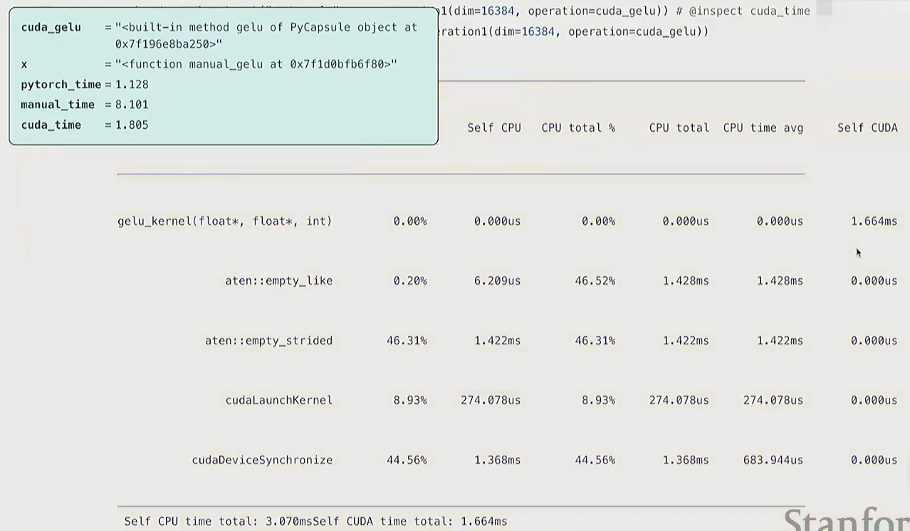
return cuda_gelu结论
- cuda实现的gelu运行时间相比于mamual有很大提升
Q:为什么manual的实现这么慢?
A:
- 并不是因为它把数据从GPU发回CPU的通信成本导致的(比如x驻留在GPU上,我们在GPU分配它,虽然我们会写
as device=cuda,但其实数据不会一直驻留在SM上)。- 而是,例如在计算x的平方时, 乘法操作会把向量从全局内存读到SMs中, 进行计算, 再写回去。所以这涉及到的是,DRAM与SMs的通信成本, 而非CPU到GPU的通信成本。
- 如果写成
as device=cpu, 就会产生CPU传输成本, 再加上DRAM传输成本。
Triton
Triton vs Cuda
| 特性 | CUDA | Triton |
|---|---|---|
| Memory coalescing (transfer from DRAM) 内存合并(从DRAM传输数据) | manual(手动) | automatic(自动) |
| Shared memory management 共享内存管理 | manual(手动) | automatic(自动) |
| Scheduling within SMs 流式多处理器(SM)内调度 | manual(手动) | automatic(自动) |
| Scheduling across SMs 流式多处理器(SM)间调度 | manual(手动) | manual(手动) |
补充说明:
- 内存合并(Memory Coalescing):GPU访问DRAM时的一种优化技术,通过让线程束(warp)内的线程访问连续内存地址,减少内存请求次数,提升数据传输效率。CUDA需开发者手动确保内存访问模式符合合并规则,Triton会自动优化该过程。
- 共享内存(Shared Memory):GPU片上高速内存,访问速度远快于DRAM,常用于线程块内数据复用。CUDA需手动分配、读写和释放共享内存,Triton会根据代码逻辑自动管理。
- 流式多处理器(SM):GPU的核心计算单元(如NVIDIA GPU的SM、AMD GPU的CU),一个GPU包含多个SM。"SM内调度"指同一SM内线程/线程块的执行顺序优化,"SM间调度"指不同SM间的任务分配,后者因涉及GPU硬件资源全局分配,目前CUDA和Triton均需手动干预(或依赖框架高层调度)。
triton的gelu实现
python
@triton.jit
def triton_gelu_kernel(x_ptr, y_ptr, num_elements, BLOCK_SIZE: tl.constexpr):
    """
    Triton核函数:实现GELU激活函数的并行计算
    由triton.jit装饰器编译为高效GPU代码,自动优化内存访问和线程调度

    参数:
        x_ptr: 输入张量的数据指针(GPU内存)
        y_ptr: 输出张量的数据指针(GPU内存)
        num_elements: 输入张量的总元素数量
        BLOCK_SIZE: 每个线程块处理的元素数量(编译期常量)
    """
    # 输入数据位于x_ptr,输出结果将存储在y_ptr
    # 线程块划分示意图:
    #     |        Block 0            |          Block 1          |      ...      |
    #                            BLOCK_SIZE                                 num_elements

    # 获取当前线程块在网格中的ID(轴0方向,1D网格)
    pid = tl.program_id(axis=0)
    # 计算当前线程块处理的第一个元素索引
    block_start = pid * BLOCK_SIZE

    # 生成当前线程块内所有线程要处理的元素偏移量
    # 例如:block_start=1024, BLOCK_SIZE=1024时,offsets为[1024, 1025, ..., 2047]
    offsets = block_start + tl.arange(0, BLOCK_SIZE)

    # 创建掩码:标记哪些偏移量在有效元素范围内(处理总元素数不是BLOCK_SIZE整数倍的情况)
    mask = offsets < num_elements

    # 从全局内存加载数据到线程块寄存器
    # mask确保只加载有效元素,避免越界访问
    x = tl.load(x_ptr + offsets, mask=mask)

    # 计算GELU激活函数(近似实现)
    # 公式:GELU(x) = 0.5 * x * (1 + tanh(sqrt(2/π) * (x + 0.044715 * x³)))
    # 其中0.79788456是sqrt(2/π)的近似值

    # 计算tanh内部的表达式
    a = 0.79788456 * (x + 0.044715 * x * x * x)
    # Triton原生不直接提供tanh函数,使用等价公式:tanh(a) = (e^(2a) - 1) / (e^(2a) + 1)
    exp = tl.exp(2 * a)
    tanh = (exp - 1) / (exp + 1)
    # 计算最终GELU结果
    y = 0.5 * x * (1 + tanh)

    # 将计算结果从寄存器存储到全局内存的输出地址
    # mask确保只存储有效元素的结果
    tl.store(y_ptr + offsets, y, mask=mask)

def triton_gelu(x: torch.Tensor):
    """
    使用Triton框架实现的GELU激活函数,在GPU上高效执行

    参数:
        x: 输入张量,必须是CUDA设备上的连续张量
    返回:
        应用GELU激活函数后的输出张量,形状与输入相同
    """
    # 输入验证:确保张量在CUDA设备上(Triton kernels仅在GPU上运行)
    assert x.is_cuda
    # 输入验证:确保张量是连续内存布局(优化内存访问效率)
    assert x.is_contiguous()

    # 分配与输入形状、类型、设备相同的空张量作为输出
    y = torch.empty_like(x)

    # 确定并行计算的网格划分方式
    # 获取输入张量的总元素数量
    num_elements = x.numel()
    # 每个线程块处理的元素数量(Triton中通常设为1024,适配GPU warp大小)
    block_size = 1024
    # 计算需要的线程块数量(向上取整确保所有元素都被处理)
    num_blocks = triton.cdiv(num_elements, block_size)

    # 启动Triton kernel执行GELU计算
    # [(num_blocks,)] 定义网格维度(此处为1D网格)
    # 传递输入张量x、输出张量y、元素总数和块大小参数
    triton_gelu_kernel[(num_blocks,)](x, y, num_elements, BLOCK_SIZE=block_size)

    # 返回计算结果
    return y
PTX
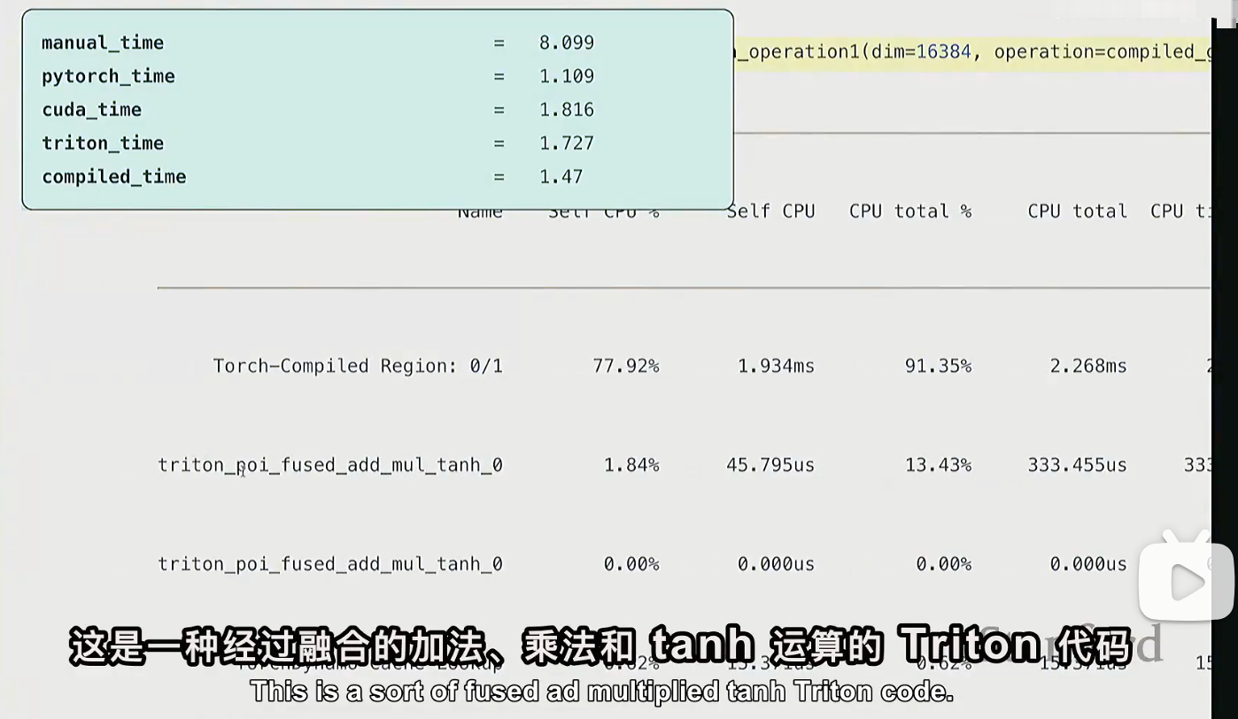
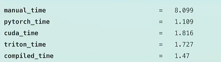
不同版本的gelu对比
python
# 直接利用torch.compile
compiled_gelu = torch.compile(manual_gelu)
torch.compile 将未经优化的代码,转为更优化的代码,会尝试自动融合算子。可以看到,底层用的是triton
不同版本的softmax
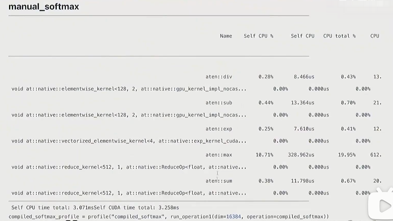
manual
python
def manual_softmax(x: torch.Tensor):
    """
    手动实现Softmax激活函数,对输入张量的每一行进行归一化处理
    Softmax公式:softmax(x)_ij = exp(x_ij) / sum(exp(x_ik) for k in 0..N-1)

    参数:
        x: 输入张量,形状为[M, N],M为样本数,N为特征数
    返回:
        y: 经过Softmax处理的张量,形状与输入相同,每行元素和为1
    """
    # 获取输入张量的形状:M为行数(样本数),N为列数(特征数)
    M, N = x.shape

    # 计算每一行的最大值(用于数值稳定性,防止指数溢出)
    # 操作:MN次读取(遍历所有元素),M次写入(存储每行最大值)
    x_max = x.max(dim=1)[0]  # [0]表示取最大值结果,忽略索引

    # 每行元素减去该行的最大值(数值稳定化步骤)
    # 操作:MN次读取(x的所有元素) + M次读取(x_max的所有元素),MN次写入(存储结果)
    # [:, None]将x_max从形状[M]扩展为[M, 1],以便与x进行广播运算
    x = x - x_max[:, None]

    # 对处理后的元素进行指数运算(计算分子)
    # 操作:MN次读取(x的所有元素),MN次写入(存储指数结果)
    numerator = torch.exp(x)

    # 计算每行的指数和(归一化常数,即分母)
    # 操作:MN次读取(numerator的所有元素),M次写入(存储每行的和)
    denominator = numerator.sum(dim=1)

    # 计算最终的Softmax结果:分子除以分母(带广播)
    # 操作:MN次读取(numerator) + M次读取(denominator),MN次写入(存储结果)
    y = numerator / denominator[:, None]

    # 内存操作统计:
    # 总读取次数:5MN + M(上述各步骤读取次数之和)
    # 总写入次数:3MN + 2M(上述各步骤写入次数之和)
    # 理论优化空间:理想情况下只需MN次读取和MN次写入(可实现4倍速提升)
    return y
triton
python
def triton_softmax(x: torch.Tensor):
    """
    使用Triton框架优化的Softmax实现,通过GPU并行计算提升性能

    参数:
        x: 输入张量,形状为[M, N],需为CUDA设备上的连续张量
    返回:
        y: 归一化后的张量,形状与输入相同
    """
    # 分配与输入形状、类型、设备相同的空张量作为输出
    y = torch.empty_like(x)

    # 确定并行计算的网格配置
    M, N = x.shape                          # M为行数,N为列数
    # 每个线程块处理一行,块大小设为大于等于列数的最小2的幂(优化内存访问)
    block_size = triton.next_power_of_2(N)
    num_blocks = M                          # 行数决定线程块数量(每个线程块处理一行)

    # 启动Triton核函数执行并行计算
    triton_softmax_kernel[(M,)](            # 网格维度:M个线程块(每行一个)
        x_ptr=x, y_ptr=y,                   # 输入输出张量指针
        x_row_stride=x.stride(0),           # 输入张量行间距(每行第一个元素的内存偏移)
        y_row_stride=y.stride(0),           # 输出张量行间距
        num_cols=N,                         # 列数(特征维度)
        BLOCK_SIZE=block_size               # 线程块大小(编译期常量)
    )

    return y


@triton.jit
def triton_softmax_kernel(x_ptr, y_ptr, x_row_stride, y_row_stride, num_cols, BLOCK_SIZE: tl.constexpr):
    """
    Triton核函数:并行计算Softmax,每个线程块处理输入张量的一行

    参数:
        x_ptr: 输入张量的数据指针(GPU内存)
        y_ptr: 输出张量的数据指针(GPU内存)
        x_row_stride: 输入张量每行的内存步长(字节数)
        y_row_stride: 输出张量每行的内存步长(字节数)
        num_cols: 每行的元素数量(特征维度)
        BLOCK_SIZE: 线程块大小(编译期常量,需>=num_cols)
    """
    # 确保线程块大小足够容纳一行的所有元素
    assert num_cols <= BLOCK_SIZE

    # 每个线程块独立处理一行,获取当前处理的行索引
    row_idx = tl.program_id(0)
    # 生成当前线程块内所有线程的列偏移量(0到BLOCK_SIZE-1)
    col_offsets = tl.arange(0, BLOCK_SIZE)

    # 计算输入张量中当前行的起始内存地址
    x_start_ptr = x_ptr + row_idx * x_row_stride
    # 计算当前行所有元素的内存地址(带列偏移)
    x_ptrs = x_start_ptr + col_offsets
    # 从全局内存加载一行数据,超出有效列数的位置用-inf填充(不影响max计算)
    # mask确保只加载有效列元素,避免越界访问
    x_row = tl.load(x_ptrs, mask=col_offsets < num_cols, other=float("-inf"))

    # 并行计算Softmax(所有操作在寄存器中完成,减少全局内存访问)
    # 1. 减去行内最大值(数值稳定化)
    x_row = x_row - tl.max(x_row, axis=0)
    # 2. 计算指数(分子)
    numerator = tl.exp(x_row)
    # 3. 计算归一化常数(分母)
    denominator = tl.sum(numerator, axis=0)
    # 4. 计算最终结果
    y_row = numerator / denominator

    # 计算输出张量中当前行的起始内存地址
    y_start_ptr = y_ptr + row_idx * y_row_stride
    # 计算当前行所有输出元素的内存地址(带列偏移)
    y_ptrs = y_start_ptr + col_offsets
    # 将计算结果存储到全局内存,只存储有效列元素
    tl.store(y_ptrs, y_row, mask=col_offsets < num_cols)
torch.compile
python
compiled_softmax = torch.compile(manual_softmax)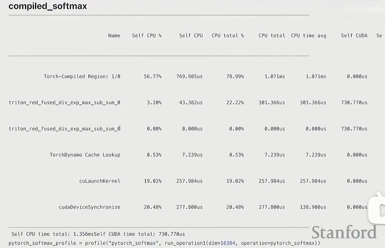
pytorch
python
def pytorch_softmax(x: torch.Tensor):
    return torch.nn.functional.softmax(x, dim=-1)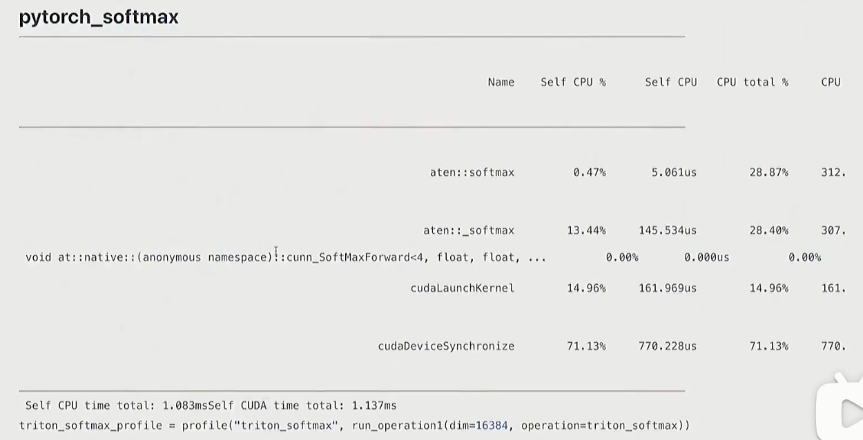
结论
- torch.compile会比pytorch实现更好
- mamual调用cuda的次数最多