4 用pytorch实现线性回归
文章目录
- [4 用pytorch实现线性回归](#4 用pytorch实现线性回归)
-
- [1 复习引入](#1 复习引入)
- [2 模型建立](#2 模型建立)
-
- [1 训练数据](#1 训练数据)
- [2 设计模型](#2 设计模型)
- [3 构造损失函数和优化器](#3 构造损失函数和优化器)
- [4 做好训练的过程](#4 做好训练的过程)
- [3 代码综合](#3 代码综合)
- 总结
-
- [1 深度学习的流程](#1 深度学习的流程)
- [2. 代码处理](#2. 代码处理)
- [3 函数总结](#3 函数总结)
-
- `torch.tensor()`
- `torch.nn.Linear()`
- [` torch.nn.MSELoss()`](#
torch.nn.MSELoss()) - `torch.optim.SGD()`
- `.zero_grad()`
- `.backward()`
- `Model.linear.weight.item()`
- `Model.linear.bias.item()`
1 复习引入
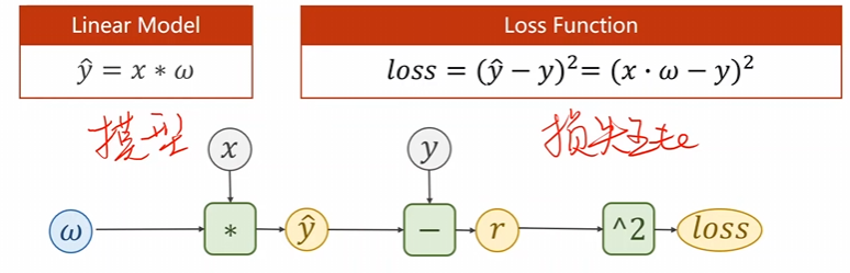
和上一次一样采用的是这个比较基本的模型进行讲解,并且采用随机下降模型梯度
在上一讲中已经使用了一定的pytorch的模型
tensor:数据backward()自动反馈求解处理。
2 模型建立
1 训练数据
给定一定的样本数据
这次咱们应当使用的是具体的pytorch的数据结构进行输入,采用的是 m i n i b a t c h mini\ batch mini batch。
也就是说将 x x x和 y y y放在一起即可。
例如: ( x 1 , y 1 ) , ( x 2 , y 2 ) , ( x 3 , y 3 ) (x_{1},y_{1}),(x_{2},y_{2}),(x_{3},y_{3}) (x1,y1),(x2,y2),(x3,y3)
python
import torch

x_data = torch.Tensor([[1.0], [2.0], [3.0]])
y_data = torch.Tensor([[2.0], [4.0], [6.0]])
注意:x和y必须是矩阵。
2 设计模型
用来计算咱们的 y ^ \hat{y} y^
根据比较基本的模型也就是线性模型而言: y ^ = w × x + b \hat{y}=w\times x + b y^=w×x+b
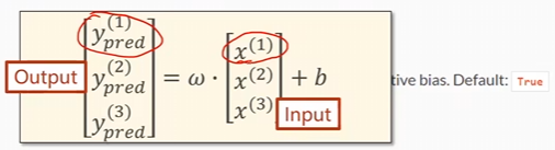
如果输入的数据是上面那个样子的话,那么咱们的 y ^ \hat{y} y^就可以变成, { y ^ 1 = w ⋅ x 1 + b y ^ 2 = w ⋅ x 2 + b y ^ 3 = w ⋅ x 3 + b \begin{cases}\hat{y}{1}=w\cdot x{1}+b\\\hat{y}{2}=w\cdot x{2}+b\\\hat{y}{3}=w\cdot x{3}+b&\end{cases} ⎩ ⎨ ⎧y^1=w⋅x1+by^2=w⋅x2+by^3=w⋅x3+b
这个时候就可以采用向量的写法了: y \^ 1 y \^ 2 y \^ 3 = w ⋅ x 1 x 2 x 3 + b \left.\left\\begin{array}{c}{\\hat{y}_{1}}\\\\{\\hat{y}_{2}}\\\\{\\hat{y}_{3}}\\end{array}\\right.\\right=w\cdot\begin{bmatrix}{x_{1}}\\{x_{2}}\\{x_{3}}\end{bmatrix}+b y^1y^2y^3 =w⋅ x1x2x3 +b
之前咱们是人工求导数 的,现在咱们最重要的事情是构造计算图 ,求导是 p y t o r c h pytorch pytorch的事情。
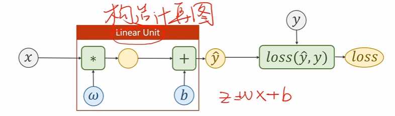
这个时需要要确定权重的性转和 b b b的大小。
如果想要知道权重的形状那么就需要知道输入的一个维度形状。
注意输出的 l o s s loss loss必须是一个标量。
在
pytorch中首先先将模型定义成一个类。每一个类一定要继承咱们的
Module模块
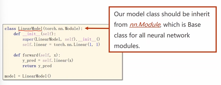
注意:必须要这两个函数,一个是
__init__()另一个是forward()名字都不可以错。
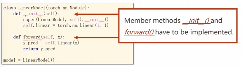
python
class LinearModel(torch.nn.Module):
    def __init__(self):
        super(LinearModel, self).__init__() # 调用副类,直接这么写就完了。
        self.linear = torch.nn.Linear(1, 1) #nn.linear()是pytorch的一个类,这两个分别是权重和偏置。也在构造一个对象。 Neural network nn.Linear(输入维度,输出维度)。

    def forward(self, x): # forward的函数名是固定的。
        y_pred = self.linear(x) #实现了一个可以调用的对象。
        return y_pred

model = LinearModel() # 实例化
nn.Linear(in_features,out_features,bias=True)
- in_features : size of each input sample
- out_features : size of each output sample
- bias : If set to False, the layer will not learn an additive bias. Default: True
python
class LinearModel(torch.nn.Module):
    def __init__(self):
        super(LinearModel, self).__init__()
        self.linear = torch.nn.Linear(1, 1)

    def forward(self, x):
        y_pred = self.linear(x)
        return y_pred

model = LinearModel()
3 构造损失函数和优化器
使用pytorch的应用接口进行构造。
咱们原本的模型为: l o s s = ( y ^ − y ) 2 loss = (\hat{y}-y)^2 loss=(y^−y)2
那么对于这么一堆数据就有: l o s s 1 = ( y ^ 1 − y 1 ) 2 l o s s 2 = ( y ^ 2 − y 2 ) 2 l o s s 3 = ( y ^ 3 − y 3 ) 2 loss_{1}=(\hat{y}{1}-y{1})^{2} \\loss_{2}=(\hat{y}{2}-y{2})^{2} \\loss_{3}=(\hat{y}{3}-y{3})^{2} loss1=(y^1−y1)2loss2=(y^2−y2)2loss3=(y^3−y3)2。
这时候用向量的形式可以表示为: log 2 log 2 log 3 = ( y \^ 1 y \^ 2 y \^ 3 − y 1 y \^ 2 y \^ 3 ) 2 \begin{bmatrix}\log_2\\\log_2\\\log_3\end{bmatrix}=\begin{pmatrix}\begin{bmatrix}\hat{y}_1\\\hat{y}_2\\\hat{y}_3\end{bmatrix}-\begin{bmatrix}y_1\\\hat{y}_2\\\hat{y}_3\end{bmatrix}\end{pmatrix}^{2} log2log2log3 = y^1y^2y^3 − y1y^2y^3 2
由于要求咱么输出的loss是一个标量,因此需要将这个 l o s s loss loss进行求和操作。
用
MSE的方式求loss这个MSEloss也是继承nn下的module,计算图
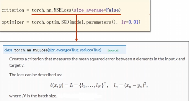
torch.nn.MSELoss(size_average = True , reduce=Ture)
- 是否需要求均值
- 是否需要计算聚合的标量损失值,所谓聚合就是求和罢了。
注意这个里面的东西已经被弃用了 现在合成了一个
reduction
reduction='mean': 等价于reduce=True且size_average=True。计算批次的平均损失。reduction='sum': 等价于reduce=True且size_average=False。计算批次的总和损失。reduction='none': 等价于reduce=False。不进行聚合,返回每个样本的损失。
优化器
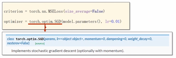
这个
parameter会检查这里面的所有成员,如果有相应的权重,那么直接就加到咱们的训练结果上面。
python
criterion = torch.nn.MSELoss(size_average=False)
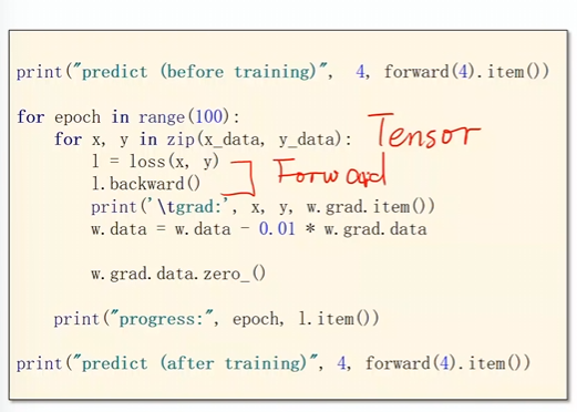
optimizer = torch.optim.SGD(model.parameters(), lr=0.01)4 做好训练的过程
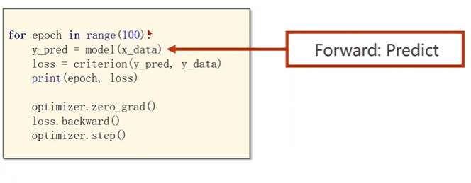
forward, backward, update,
将这个训练数据送进去
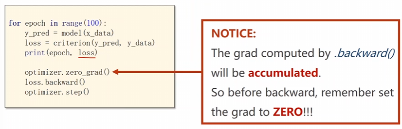
一定要注意梯度的归零操作。
然后进行反向传播
- y ^ \hat{y} y^
- l o s s loss loss
- b a c k w a r d backward backward
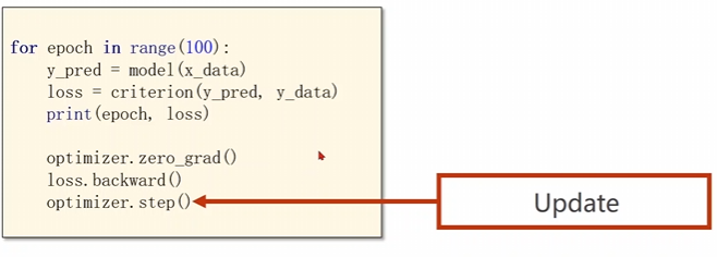
- u p a d e upade upade
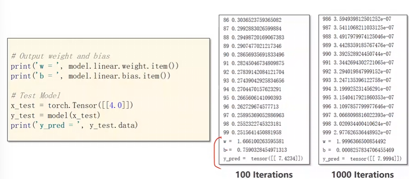
最后打印这个运行的日志。
python
for epoch in range(100):
    y_pred = model(x_data)
    loss = criterion(y_pred, y_data)
    print(epoch, loss)

    optimizer.zero_grad()
    loss.backward()
    optimizer.step()
3 代码综合
python
import numpy as np
import matplotlib.pyplot as plt
import torch
# 1 训练数据准备
x_data = torch.tensor([[1.0] , [2.0] , [3.0]])
y_data = torch.tensor([[2.0] , [4.0] , [6.0]])
# 2 设计模型 线性模型 y=x*w+b loss 求和平方函数
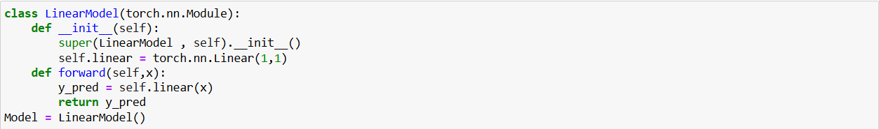
class LinearModel(torch.nn.Module):
def __init__(self):
super(LinearModel , self).__init__()
self.linear = torch.nn.Linear(1,1) # 定义线性模型 y = w*x + b
def forward(self , x):
y_pred = self.linear(x) # 直节调用self.linear()这个方法
return y_pred
Model = LinearModel() # 模型进行实例化
# 3 定义损失函数并确定优化器
criterion = torch.nn.MSELoss(size_average=False) # sum
optimizer = torch.optim.SGD(Model.parameters(),lr =0.05)
# 4 开始进行学习
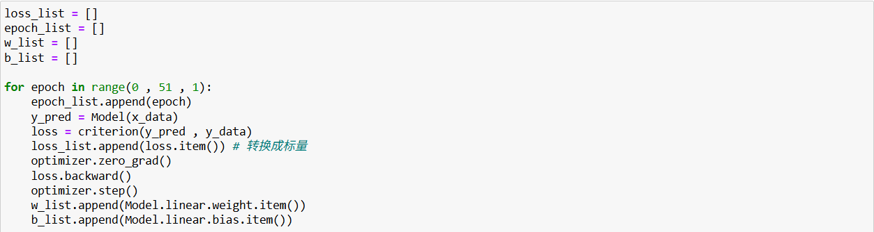
loss_list = []
epoch_list = []
w_list = []
b_list = []
for epoch in range(0 , 51 , 1):
epoch_list.append(epoch)
y_pred = Model(x_data)
loss = criterion(y_pred , y_data)
loss_list.append(loss.item()) # 转换成标量
optimizer.zero_grad()
loss.backward()
optimizer.step()
w_list.append(Model.linear.weight.item())
b_list.append(Model.linear.bias.item())
# 日志打印
for e,l,w ,b in zip(epoch_list , loss_list , w_list , b_list):
print(f'第{e}轮的时候,损失为{l:.6f},权重为{w:.6f} , 偏置为{b:.6f} \n')
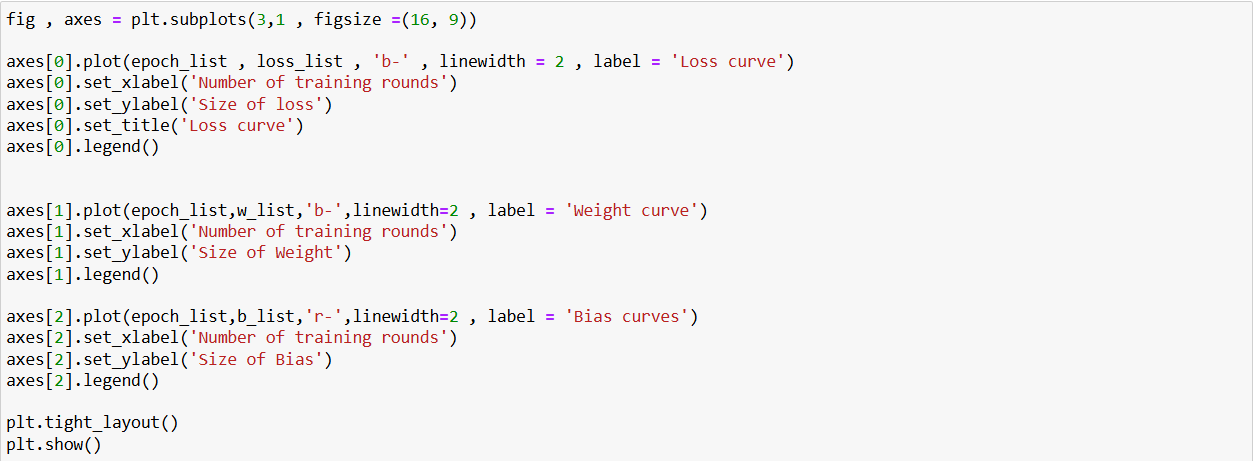
fig , axes = plt.subplots(3,1 , figsize =(5, 6))
axes[0].plot(epoch_list , loss_list , 'b-' , linewidth = 2 , label = 'Loss curve')
axes[0].set_xlabel('Number of training rounds')
axes[0].set_ylabel('Size of loss')
axes[0].set_title('Loss curve')
axes[0].legend()
axes[1].plot(epoch_list,w_list,'b-',linewidth=2 , label = 'Weight curve')
axes[1].set_xlabel('Number of training rounds')
axes[1].set_ylabel('Size of Weight')
axes[1].legend()
axes[2].plot(epoch_list,b_list,'r-',linewidth=2 , label = 'Bias curves')
axes[2].set_xlabel('Number of training rounds')
axes[2].set_ylabel('Size of Bias')
axes[2].legend()
plt.tight_layout()
plt.show()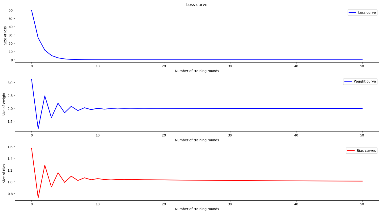
注意
pytorch有很多优化器:
- torch.optim.Adagrad
- torch.optim.Adam
- torch.optim.Adamax
- torch.optim.ASGD
- torch.optim.LBFGS
- torch.optim.RMSprop
- torch.optim.Rprop
- torch.optim.SGD
总结
这一次咱们主要使用了pytorch进行线性模型的学习操作,让我们再一次回顾一下各类操作,以及深度学习的流程。
1 深度学习的流程
实际上深度学习的流程就那么四个
- 确定并导入训练数据。
- 确定并设计训练模型。
- 给定损失函数以及优化器。
- 进行训练,打印日志,绘制图表。
2. 代码处理
根据上面四部,我们再一次比较清晰粗略的以线性模型为例子,进行说明。
1 确定并导入训练模型。

2 确定并设计训练模型。
3 给定损失函数以及优化器。

4 进行训练
打印日志

绘制图表
可见其实使用pytorch进行深度学习是非常的清晰的。我们最终要的就是对其中的第二步 和第三步进行琢磨和处理。
3 函数总结
最后的最后让我把这一次使用到的函数进行一个总结
torch.tensor()
创建一个PyTorch张量(Tensor),这是PyTorch中最基本的数据结构。
- 类似于NumPy的ndarray,但可以在GPU上运行
- 支持自动求导(Autograd)
- 是深度学习计算的基础单元
torch.nn.Linear()
创建一个全连接层(线性层),执行线性变换:y = xA^T + b
参数:
-
in_features:输入特征数 -
out_features:输出特征数 -
bias:是否使用偏置项(默认为True)
内部参数:
.weight:权重矩阵,形状为(out_features, in_features).bias:偏置向量,形状为(out_features,)
torch.nn.MSELoss()
算均方误差损失 ( M e a n S q u a r e d E r r o r L o s s ) (Mean Squared Error Loss) (MeanSquaredErrorLoss),用于回归问题。
公式 : M S E = 1 N ∑ i = 1 N ( y i − y ^ i ) 2 \mathrm{MSE}=\frac{1}{N}\sum_{i=1}^N(y_i-\hat{y}_i)^2 MSE=N1∑i=1N(yi−y^i)2
参数:
reduction:指定缩减方式'mean':返回损失的均值(默认)'sum':返回损失的总和'none':不缩减,返回每个元素的损失
torch.optim.SGD()
实现随机梯度下降优化算法。
参数:
params:需要优化的参数(通常来自model.parameters())lr:学习率(learning rate)momentum:动量系数(可选,默认为0)weight_decay:权重衰减(L2正则化,可选)
.zero_grad()
将模型参数的梯度清零。
.backward()
自动计算梯度(反向传播)
Model.linear.weight.item()
从权重张量中提取标量值。
分解:
Model.linear:访问模型中的linear层.weight:获取该层的权重参数(是一个张量).item():将单元素张量转换为Python标量
Model.linear.bias.item()
从偏置张量中提取标量值。
分解:
Model.linear:访问模型中的linear层.bias:获取该层的偏置参数(是一个张量).item():将单元素张量转换为Python标量