文章目录
- 绘图类型
- 成对数据
- [plot(x, y)](#plot(x, y))
- [scatter(x, y)](#scatter(x, y))
- [bar(x, height)](#bar(x, height))
- [stem(x, y)](#stem(x, y))
- [fill_between(x, y1, y2)](#fill_between(x, y1, y2))
- [stackplot(x, y)](#stackplot(x, y))
- stairs(values)
- 统计分布
- hist(x)
- boxplot(X)
- [errorbar(x, y, yerr, xerr)](#errorbar(x, y, yerr, xerr))
- 小提琴图绘制指南
- eventplot(D)
- [hist2d(x, y)](#hist2d(x, y))
- [hexbin(x, y, C)](#hexbin(x, y, C))
- pie(x)
- ecdf(x)
- 网格数据
- imshow(Z)
- [pcolormesh(X, Y, Z)](#pcolormesh(X, Y, Z))
- [contour(X, Y, Z)](#contour(X, Y, Z))
- [contourf(X, Y, Z)](#contourf(X, Y, Z))
- [barbs(X, Y, U, V)](#barbs(X, Y, U, V))
- [quiver(X, Y, U, V)](#quiver(X, Y, U, V))
- [streamplot(X, Y, U, V)](#streamplot(X, Y, U, V))
- 非规则网格数据
- [tricontour(x, y, z)](#tricontour(x, y, z))
- [tricontourf(x, y, z)](#tricontourf(x, y, z))
- [tripcolor(x, y, z)](#tripcolor(x, y, z))
- [triplot(x, y)](#triplot(x, y))
- 三维与体积数据可视化
- [bar3d(x, y, z, dx, dy, dz)](#bar3d(x, y, z, dx, dy, dz))
- [fill_between(x1, y1, z1, x2, y2, z2)](#fill_between(x1, y1, z1, x2, y2, z2))
- [plot(xs, ys, zs)](#plot(xs, ys, zs))
- [quiver(X, Y, Z, U, V, W)](#quiver(X, Y, Z, U, V, W))
- [scatter(xs, ys, zs)](#scatter(xs, ys, zs))
- [stem(x, y, z)](#stem(x, y, z))
- [plot_surface(X, Y, Z)](#plot_surface(X, Y, Z))
- [plot_trisurf(x, y, z)](#plot_trisurf(x, y, z))
- [voxels(\x, y, z, filled)](#voxels([x, y, z], filled))
- [plot_wireframe(X, Y, Z)](#plot_wireframe(X, Y, Z))
绘图类型
https://matplotlib.org/stable/plot_types/index.html
Matplotlib 提供的多种常见绘图命令概览。
成对数据
展示成对数据 \((x, y))、表格数据 \((var_0, \cdots, var_n)) 以及函数数据 \(f(x)=y) 的图表。
plot(x, y)
scatter(x, y)
bar(x, height)
stem(x, y)
fill_between(x, y1, y2)
stackplot(x, y)
stairs(values)
统计分布
展示数据集中至少一个变量的分布情况。部分方法还会计算分布特征。
hist(x)
boxplot(X)
errorbar(x, y, yerr, xerr)
violinplot(D)
eventplot(D)
hist2d(x, y)
hexbin(x, y, C)
pie(x)
ecdf(x)
网格化数据
展示数组和图像 \(Z_{i, j}) 以及场数据 \(U_{i, j}, V_{i, j}) 在规则网格上的可视化效果,以及对应的坐标网格 \(X_{i,j}, Y_{i,j})。
imshow(Z)
pcolormesh(X, Y, Z)

contour(X, Y, Z)

contourf(X, Y, Z)
barbs(X, Y, U, V)
quiver(X, Y, U, V)
streamplot(X, Y, U, V)
非规则网格数据
绘制在非结构化网格上的数据\(Z_{x, y})、非结构化坐标网格\((x, y))以及二维函数\(f(x, y) = z)的图表。
tricontour(x, y, z)
tricontourf(x, y, z)
tripcolor(x, y, z)

triplot(x, y)
三维与体数据可视化
使用 mpl_toolkits.mplot3d 库绘制三维坐标点 \((x,y,z))、曲面函数 \(f(x,y)=z) 以及体数据 \(V_{x, y, z}) 的可视化图表。
bar3d(x, y, z, dx, dy, dz)
fill_between(x1, y1, z1, x2, y2, z2)
fill_between(x1, y1, z1, x2, y2, z2)
plot(xs, ys, zs)
quiver(X, Y, Z, U, V, W)
scatter(xs, ys, zs)
stem(x, y, z)
plot_surface(X, Y, Z)
plot_trisurf(x, y, z)
voxels(\[x, y, z, filled)](https://matplotlib.org/stable/plot_types/3D/voxels_simple.html#sphx-glr-plot-types-3d-voxels-simple-py)
voxels(x, y, z, filled)
plot_wireframe(X, Y, Z)
- [
下载所有Python源码示例: plot_types_python.zip: https://matplotlib.org/stable/_downloads/ea73be0751ffd403489ec6af7a17ed2c/plot_types_python.zip - [
下载所有Jupyter笔记本示例: plot_types_jupyter.zip: https://matplotlib.org/stable/_downloads/4e1270d363927f553fd952d7a2603176/plot_types_jupyter.zip
成对数据
https://matplotlib.org/stable/plot_types/basic/index.html
展示成对数据 \((x, y))、表格数据 \((var_0, \cdots, var_n)) 以及函数数据 \(f(x)=y) 的图表。
plot(x, y)
scatter(x, y)
bar(x, height)
stem(x, y)
fill_between(x, y1, y2)
stackplot(x, y)
stairs(values)
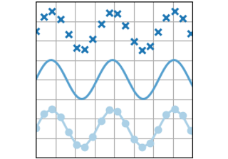
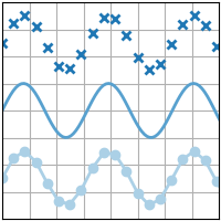
plot(x, y)
https://matplotlib.org/stable/plot_types/basic/plot.html
绘制 y 相对于 x 的线条和/或标记图。
详情参阅 plot 文档。
python
import matplotlib.pyplot as plt
import numpy as np

plt.style.use('_mpl-gallery')

# make data
x= np.linspace(0, 10, 100)
y= 4 + 1 * np.sin(2 * x)
x2 = np.linspace(0, 10, 25)
y2 = 4 + 1 * np.sin(2 * x2)

# plot
fig, ax = plt.subplots()

ax.plot(x2, y2 + 2.5, 'x', markeredgewidth=2)
ax.plot(x, y, linewidth=2.0)
ax.plot(x2, y2 - 2.5, 'o-', linewidth=2)

ax.set(xlim=(0, 8), xticks=np.arange(1, 8),
       ylim=(0, 8), yticks=np.arange(1, 8))

plt.show()- 下载 Jupyter 笔记本:
plot.ipynb: https://matplotlib.org/stable/_downloads/c3549a960f949135fab7fae6e7db2e7e/plot.ipynb - 下载 Python 源代码:
plot.py: https://matplotlib.org/stable/_downloads/87d4c90a7e5e6ca21ec5cc86b40a553a/plot.py - 下载压缩包:
plot.zip: https://matplotlib.org/stable/_downloads/edf936f9c842f4fff92a25655e5bd78d/plot.zip
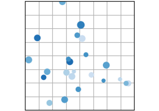
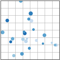
scatter(x, y)
https://matplotlib.org/stable/plot_types/basic/scatter_plot.html
散点图,展示 y 随 x 的变化关系,支持调整标记点的大小和/或颜色。
详情参阅 scatter。
python
import matplotlib.pyplot as plt
import numpy as np

plt.style.use('_mpl-gallery')

# make the data
np.random.seed(3)
x= 4 + np.random.normal(0, 2, 24)
y= 4 + np.random.normal(0, 2, len(x))
# size and color:
sizes = np.random.uniform(15, 80, len(x))
colors = np.random.uniform(15, 80, len(x))

# plot
fig, ax = plt.subplots()

ax.scatter(x, y, s=sizes, c=colors, vmin=0, vmax=100)

ax.set(xlim=(0, 8), xticks=np.arange(1, 8),
       ylim=(0, 8), yticks=np.arange(1, 8))

plt.show()- 下载 Jupyter 笔记本:
scatter_plot.ipynb: https://matplotlib.org/stable/_downloads/43385562b6168494e9464fd4ea79d5be/scatter_plot.ipynb - 下载 Python 源代码:
scatter_plot.py: https://matplotlib.org/stable/_downloads/f6c5e42b48428d3790657a757dda91a5/scatter_plot.py - 下载压缩包:
scatter_plot.zip: https://matplotlib.org/stable/_downloads/fa4d52647b36a4f0ad2cde0a62b9d949/scatter_plot.zip
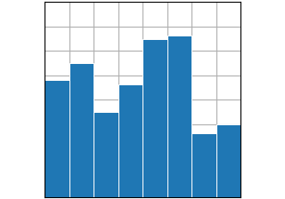
bar(x, height)
https://matplotlib.org/stable/plot_types/basic/bar.html
参见 bar。

python
import matplotlib.pyplot as plt
import numpy as np

plt.style.use('_mpl-gallery')

# make data:
x= 0.5 + np.arange(8)
y = [4.8, 5.5, 3.5, 4.6, 6.5, 6.6, 2.6, 3.0]

# plot
fig, ax = plt.subplots()

ax.bar(x, y, width=1, edgecolor="white", linewidth=0.7)

ax.set(xlim=(0, 8), xticks=np.arange(1, 8),
       ylim=(0, 8), yticks=np.arange(1, 8))

plt.show()- 下载 Jupyter 笔记本:
bar.ipynb: https://matplotlib.org/stable/_downloads/e4ba394a3ddfb22ccc50a8047f9a32b3/bar.ipynb - 下载 Python 源代码:
bar.py: https://matplotlib.org/stable/_downloads/b399863c18129a77916d4c8398e5b9d0/bar.py - 下载压缩包:
bar.zip: https://matplotlib.org/stable/_downloads/3979fb221dd3c27a1b95083bff355792/bar.zip
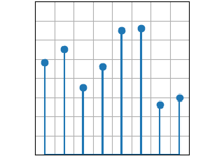
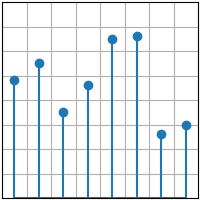
stem(x, y)
https://matplotlib.org/stable/plot_types/basic/stem.html
创建茎干图。
参见 stem。
python
import matplotlib.pyplot as plt
import numpy as np

plt.style.use('_mpl-gallery')

# make data
x= 0.5 + np.arange(8)
y = [4.8, 5.5, 3.5, 4.6, 6.5, 6.6, 2.6, 3.0]

# plot
fig, ax = plt.subplots()

ax.stem(x, y)

ax.set(xlim=(0, 8), xticks=np.arange(1, 8),
       ylim=(0, 8), yticks=np.arange(1, 8))

plt.show()- 下载 Jupyter 笔记本:
stem.ipynb: https://matplotlib.org/stable/_downloads/aa35bdc9aff50d49c3a4fb2d5766983c/stem.ipynb - 下载 Python 源代码:
stem.py: https://matplotlib.org/stable/_downloads/b6cf92aa876a4b1fda00b5f08184f673/stem.py - 下载压缩包:
stem.zip: https://matplotlib.org/stable/_downloads/90861ca691fb669a2d621db25aaf7b61/stem.zip
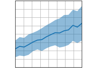
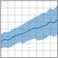
fill_between(x, y1, y2)
https://matplotlib.org/stable/plot_types/basic/fill_between.html
填充两条水平曲线之间的区域。
详情参阅 fill_between。
python
import matplotlib.pyplot as plt
import numpy as np

plt.style.use('_mpl-gallery')

# make data
np.random.seed(1)
x= np.linspace(0, 8, 16)
y1= 3 + 4*x/8 + np.random.uniform(0.0, 0.5, len(x))
y2 = 1 + 2*x/8 + np.random.uniform(0.0, 0.5, len(x))

# plot
fig, ax = plt.subplots()

ax.fill_between(x, y1, y2, alpha=.5, linewidth=0)
ax.plot(x, (y1+ y2)/2, linewidth=2)

ax.set(xlim=(0, 8), xticks=np.arange(1, 8),
       ylim=(0, 8), yticks=np.arange(1, 8))

plt.show()- 下载 Jupyter 笔记本:
fill_between.ipynb: https://matplotlib.org/stable/_downloads/0844acc3d8c8d457bc5f707c80e65bd1/fill_between.ipynb - 下载 Python 源代码:
fill_between.py: https://matplotlib.org/stable/_downloads/4db15b51c35991a3ee69725d94bb7e1c/fill_between.py - 下载压缩包:
fill_between.zip: https://matplotlib.org/stable/_downloads/b0ffe9aeda41b3ac5c4f44382b921f23/fill_between.zip
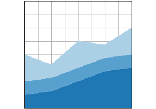
stackplot(x, y)
https://matplotlib.org/stable/plot_types/basic/stackplot.html
绘制堆叠面积图或流图。
详情参阅 stackplot

python
import matplotlib.pyplot as plt
import numpy as np

plt.style.use('_mpl-gallery')

# make data
x= np.arange(0, 10, 2)
ay = [1, 1.25, 2, 2.75, 3]
by = [1, 1, 1, 1, 1]
cy = [2, 1, 2, 1, 2]
y= np.vstack([ay, by, cy])

# plot
fig, ax = plt.subplots()

ax.stackplot(x, y)

ax.set(xlim=(0, 8), xticks=np.arange(1, 8),
       ylim=(0, 8), yticks=np.arange(1, 8))

plt.show()- 下载 Jupyter 笔记本:
stackplot.ipynb: https://matplotlib.org/stable/_downloads/93375277e615fce6a8ef8e4b02d95018/stackplot.ipynb - 下载 Python 源代码:
stackplot.py: https://matplotlib.org/stable/_downloads/b722ff173d4996c1a939d4e0d442adff/stackplot.py - 下载压缩包:
stackplot.zip: https://matplotlib.org/stable/_downloads/a04480535ada164277b11516ef1f9019/stackplot.zip
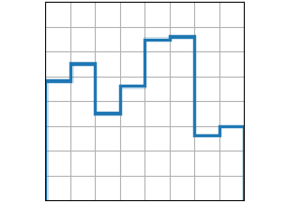
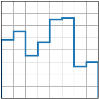
stairs(values)
https://matplotlib.org/stable/plot_types/basic/stairs.html
绘制阶梯状常数函数,可选择以线条或填充区域形式呈现。
当需要在区间\((x_i, x_{i+1}))内绘制\(y)值时,请参考stairs方法。若需在\(x)点处绘制\(y)值,请使用step方法。
python
import matplotlib.pyplot as plt
import numpy as np

plt.style.use('_mpl-gallery')

# make data
y = [4.8, 5.5, 3.5, 4.6, 6.5, 6.6, 2.6, 3.0]

# plot
fig, ax = plt.subplots()

ax.stairs(y, linewidth=2.5)

ax.set(xlim=(0, 8), xticks=np.arange(1, 8),
       ylim=(0, 8), yticks=np.arange(1, 8))

plt.show()[下载 Jupyter 笔记本文件: stairs.ipynb : https://matplotlib.org/stable/_downloads/1b052bbfe9e6d6248dc225ff7df9ca18/stairs.ipynb
- 下载 Python 源代码:
stairs.py: https://matplotlib.org/stable/_downloads/008c73d5ac1c4af82c0b90fde922ebb9/stairs.py - 下载压缩包:
stairs.zip: https://matplotlib.org/stable/_downloads/f68e38787ce561d0f194913418f19c5c/stairs.zip
统计分布
https://matplotlib.org/stable/plot_types/stats/index.html
展示数据集中至少一个变量的分布情况。部分方法还会计算分布特征。
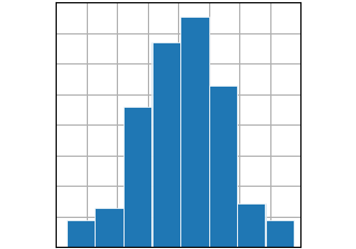
hist(x)
boxplot(X)
errorbar(x, y, yerr, xerr)
violinplot(D)
eventplot(D)
hist2d(x, y)
hexbin(x, y, C)
pie(x)
ecdf(x)
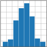
hist(x)
https://matplotlib.org/stable/plot_types/stats/hist_plot.html
计算并绘制直方图。
详情参阅 hist。
python
import matplotlib.pyplot as plt
import numpy as np

plt.style.use('_mpl-gallery')

# make data
np.random.seed(1)
x= 4 + np.random.normal(0, 1.5, 200)

# plot:
fig, ax = plt.subplots()

ax.hist(x, bins=8, linewidth=0.5, edgecolor="white")

ax.set(xlim=(0, 8), xticks=np.arange(1, 8),
       ylim=(0, 56), yticks=np.linspace(0, 56, 9))

plt.show()- 下载 Jupyter 笔记本:
hist_plot.ipynb: https://matplotlib.org/stable/_downloads/721e3406f8136c90efcd9d5508b8fcbb/hist_plot.ipynb - 下载 Python 源代码:
hist_plot.py: https://matplotlib.org/stable/_downloads/4b0bfc86a1ba58f96b40478cc4e5bb49/hist_plot.py - 下载压缩包:
hist_plot.zip: https://matplotlib.org/stable/_downloads/4978dc75c5e2b7eb3d21e66de6c06891/hist_plot.zip
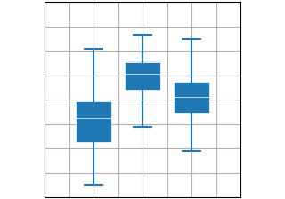
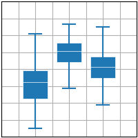
boxplot(X)
https://matplotlib.org/stable/plot_types/stats/boxplot_plot.html
绘制箱线图。
详情参见 boxplot。
python
import matplotlib.pyplot as plt
import numpy as np

plt.style.use('_mpl-gallery')

# make data:
np.random.seed(10)
D = np.random.normal((3, 5, 4), (1.25, 1.00, 1.25), (100, 3))

# plot
fig, ax = plt.subplots()
VP = ax.boxplot(D, positions=[2, 4, 6], widths=1.5, patch_artist=True,
                showmeans=False, showfliers=False,
                medianprops={"color": "white", "linewidth": 0.5},
                boxprops={"facecolor": "C0", "edgecolor": "white",
                          "linewidth": 0.5},
                whiskerprops={"color": "C0", "linewidth": 1.5},
                capprops={"color": "C0", "linewidth": 1.5})

ax.set(xlim=(0, 8), xticks=np.arange(1, 8),
       ylim=(0, 8), yticks=np.arange(1, 8))

plt.show()- 下载 Jupyter 笔记本:
boxplot_plot.ipynb: https://matplotlib.org/stable/_downloads/474e956909497683b49d4551bd2b5a8a/boxplot_plot.ipynb - 下载 Python 源代码:
boxplot_plot.py: https://matplotlib.org/stable/_downloads/c4fed0d1844aa480572cb604997e8f0d/boxplot_plot.py - 下载压缩包:
boxplot_plot.zip: https://matplotlib.org/stable/_downloads/b8a78d64658b786e4e637140d114decc/boxplot_plot.zip
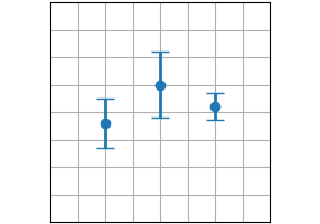
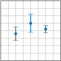
errorbar(x, y, yerr, xerr)
https://matplotlib.org/stable/plot_types/stats/errorbar_plot.html
绘制带有误差条的y对x的线图和/或标记图。
参见 errorbar。
python
import matplotlib.pyplot as plt
import numpy as np

plt.style.use('_mpl-gallery')

# make data:
np.random.seed(1)
x = [2, 4, 6]
y = [3.6, 5, 4.2]
yerr = [0.9, 1.2, 0.5]

# plot:
fig, ax = plt.subplots()

ax.errorbar(x, y, yerr, fmt='o', linewidth=2, capsize=6)

ax.set(xlim=(0, 8), xticks=np.arange(1, 8),
       ylim=(0, 8), yticks=np.arange(1, 8))

plt.show()- 下载 Jupyter 笔记本:
errorbar_plot.ipynb: https://matplotlib.org/stable/_downloads/0791d1d23a687fbe5f0916bf1e77a3a1/errorbar_plot.ipynb - 下载 Python 源代码:
errorbar_plot.py: https://matplotlib.org/stable/_downloads/10e00aece1dc1fd5bcef726cece1fb79/errorbar_plot.py - 下载压缩包:
errorbar_plot.zip: https://matplotlib.org/stable/_downloads/643dd0b572da44bb948ded3a17344bab/errorbar_plot.zip
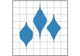
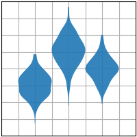
小提琴图绘制指南
https://matplotlib.org/stable/plot_types/stats/violin.html
绘制小提琴图。
API 详情参阅 violinplot。
python
import matplotlib.pyplot as plt
import numpy as np

plt.style.use('_mpl-gallery')

# make data:
np.random.seed(10)
D = np.random.normal((3, 5, 4), (0.75, 1.00, 0.75), (200, 3))

# plot:
fig, ax = plt.subplots()

vp = ax.violinplot(D, [2, 4, 6], widths=2,
                   showmeans=False, showmedians=False, showextrema=False)
# styling: for body in vp['bodies']:
    body.set_alpha(0.9)
ax.set(xlim=(0, 8), xticks=np.arange(1, 8),
       ylim=(0, 8), yticks=np.arange(1, 8))

plt.show()
下载 Jupyter 笔记本文件:violin.ipynb
下载 Python 源代码文件:violin.py
下载压缩包文件:violin.zip(https://matplotlib.org/stable/_downloads/25e3d8683ff1d01a46d298bac7568bc7/violin.zip\>
图库由 Sphinx-Gallery 生成
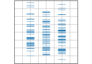
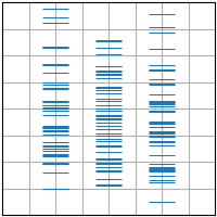
eventplot(D)
https://matplotlib.org/stable/plot_types/stats/eventplot.html
在给定位置绘制相同的平行线。
详情参阅 eventplot。
python
import matplotlib.pyplot as plt
import numpy as np

plt.style.use('_mpl-gallery')

# make data:
np.random.seed(1)
x = [2, 4, 6]
D = np.random.gamma(4, size=(3, 50))

# plot:
fig, ax = plt.subplots()

ax.eventplot(D, orientation="vertical", lineoffsets=x, linewidth=0.75)

ax.set(xlim=(0, 8), xticks=np.arange(1, 8),
       ylim=(0, 8), yticks=np.arange(1, 8))

plt.show()- 下载 Jupyter 笔记本:
eventplot.ipynb: https://matplotlib.org/stable/_downloads/9221cb78e333a9ede94fd29917ae5973/eventplot.ipynb - 下载 Python 源代码:
eventplot.py: https://matplotlib.org/stable/_downloads/68a4b2dbac0235d0eb62c070990bd582/eventplot.py - 下载压缩包:
eventplot.zip: https://matplotlib.org/stable/_downloads/b2669d063d1d2c229380b75fd0ffceda/eventplot.zip
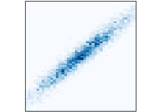
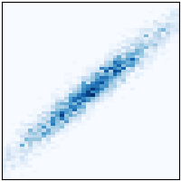
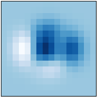
hist2d(x, y)
https://matplotlib.org/stable/plot_types/stats/hist2d.html
绘制二维直方图。
查看 hist2d 文档。
python
import matplotlib.pyplot as plt
import numpy as np

plt.style.use('_mpl-gallery-nogrid')

# make data: correlated + noise
np.random.seed(1)
x= np.random.randn(5000)
y= 1.2 * x+ np.random.randn(5000) / 3

# plot:
fig, ax = plt.subplots()

ax.hist2d(x, y, bins=(np.arange(-3, 3, 0.1), np.arange(-3, 3, 0.1)))

ax.set(xlim=(-2, 2), ylim=(-3, 3))

plt.show()- 下载 Jupyter 笔记本:
hist2d.ipynb: https://matplotlib.org/stable/_downloads/28d5ab153586d48cc859317980c33ea2/hist2d.ipynb - 下载 Python 源代码:
hist2d.py: https://matplotlib.org/stable/_downloads/1c65b20cba3b1e61c5050dac2745529f/hist2d.py - 下载压缩包:
hist2d.zip: https://matplotlib.org/stable/_downloads/c7eba7a60c4e807ee93fb5a869ff05ae/hist2d.zip
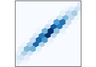
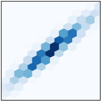
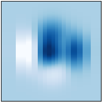
hexbin(x, y, C)
https://matplotlib.org/stable/plot_types/stats/hexbin.html
生成点集x, y的二维六边形分箱图。
详情参阅 hexbin 文档。
python
import matplotlib.pyplot as plt
import numpy as np

plt.style.use('_mpl-gallery-nogrid')

# make data: correlated + noise
np.random.seed(1)
x= np.random.randn(5000)
y= 1.2 * x+ np.random.randn(5000) / 3

# plot:
fig, ax = plt.subplots()

ax.hexbin(x, y, gridsize=20)

ax.set(xlim=(-2, 2), ylim=(-3, 3))

plt.show()- 下载 Jupyter 笔记本:
hexbin.ipynb: https://matplotlib.org/stable/_downloads/6e05805f47b2292d7de2d61ebde03410/hexbin.ipynb - 下载 Python 源代码:
hexbin.py: https://matplotlib.org/stable/_downloads/56b7bf491b1d106143dcc5df38c73d04/hexbin.py - 下载压缩包:
hexbin.zip: https://matplotlib.org/stable/_downloads/1de5e08278464fb84666eb0cfbaac64b/hexbin.zip
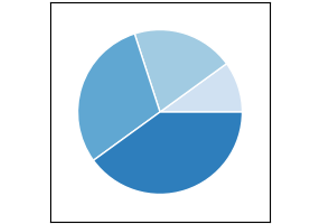
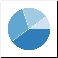
pie(x)
https://matplotlib.org/stable/plot_types/stats/pie.html
绘制饼图。
查看 pie 函数文档。
python
import matplotlib.pyplot as plt
import numpy as np

plt.style.use('_mpl-gallery-nogrid')

# make data
x = [1, 2, 3, 4]
colors = plt.get_cmap('Blues')(np.linspace(0.2, 0.7, len(x)))

# plot
fig, ax = plt.subplots()
ax.pie(x, colors=colors, radius=3, center=(4, 4),
       wedgeprops={"linewidth": 1, "edgecolor": "white"}, frame=True)

ax.set(xlim=(0, 8), xticks=np.arange(1, 8),
       ylim=(0, 8), yticks=np.arange(1, 8))

plt.show()- 下载 Jupyter 笔记本:
pie.ipynb: https://matplotlib.org/stable/_downloads/2fa20d04c4fbe9b7d334fcfd7c507390/pie.ipynb - 下载 Python 源代码:
pie.py: https://matplotlib.org/stable/_downloads/f29f319fc4f61757834bdd1ed1c80f4f/pie.py - 下载压缩包:
pie.zip: https://matplotlib.org/stable/_downloads/104cf3289bc8934cf473db7a6075f1dc/pie.zip
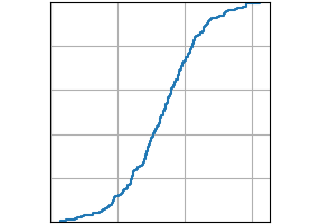
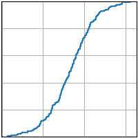
ecdf(x)
https://matplotlib.org/stable/plot_types/stats/ecdf.html
计算并绘制x的经验累积分布函数。
详情参见 ecdf。
python
import matplotlib.pyplot as plt
import numpy as np

plt.style.use('_mpl-gallery')

# make data
np.random.seed(1)
x= 4 + np.random.normal(0, 1.5, 200)

# plot:
fig, ax = plt.subplots()
ax.ecdf(x)
plt.show()- 下载 Jupyter 笔记本:
ecdf.ipynb: https://matplotlib.org/stable/_downloads/99856eef4309cd4b9e54885dc2658405/ecdf.ipynb - 下载 Python 源代码:
ecdf.py: https://matplotlib.org/stable/_downloads/12862425b3d5700010f8f1448569b890/ecdf.py - 下载压缩包:
ecdf.zip: https://matplotlib.org/stable/_downloads/1820b422f77fe6a00fac9d04a3ba5dba/ecdf.zip
网格数据
https://matplotlib.org/stable/plot_types/arrays/index.html
展示数组和图像 \(Z_{i, j}) 以及场量 \(U_{i, j}, V_{i, j}) 在规则网格上的绘图,以及对应的坐标网格 \(X_{i,j}, Y_{i,j})。
imshow(Z)
pcolormesh(X, Y, Z)
contour(X, Y, Z)
contourf(X, Y, Z)
barbs(X, Y, U, V)
quiver(X, Y, U, V)
streamplot(X, Y, U, V)
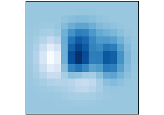
imshow(Z)
https://matplotlib.org/stable/plot_types/arrays/imshow.html
将数据显示为图像,即在二维规则栅格上呈现。
参见 imshow。
python
import matplotlib.pyplot as plt
import numpy as np

plt.style.use('_mpl-gallery-nogrid')

# make data
X, Y = np.meshgrid(np.linspace(-3, 3, 16), np.linspace(-3, 3, 16))
Z = (1 - X/2 + X**5 + Y**3) * np.exp(-X**2 - Y**2)

# plot
fig, ax = plt.subplots()

ax.imshow(Z, origin='lower')

plt.show()- 下载 Jupyter 笔记本:
imshow.ipynb: https://matplotlib.org/stable/_downloads/086e6bc8625886d5d0f79235622991ac/imshow.ipynb - 下载 Python 源代码:
imshow.py: https://matplotlib.org/stable/_downloads/553b241dfadd69049f1cb8b009914d00/imshow.py - 下载压缩包:
imshow.zip: https://matplotlib.org/stable/_downloads/ed16aaa233997a936431a9ed7605565f/imshow.zip
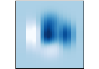
pcolormesh(X, Y, Z)
https://matplotlib.org/stable/plot_types/arrays/pcolormesh.html
创建一个非规则矩形网格的伪彩色图。
pcolormesh 比 imshow 更灵活,因为其x和y向量不需要等距分布(实际上可以是倾斜的)。
python
import matplotlib.pyplot as plt
import numpy as np

plt.style.use('_mpl-gallery-nogrid')

# make data with uneven sampling in x
x = [-3, -2, -1.6, -1.2, -.8, -.5, -.2, .1, .3, .5, .8, 1.1, 1.5, 1.9, 2.3, 3]
X, Y = np.meshgrid(x, np.linspace(-3, 3, 128))
Z = (1 - X/2 + X**5 + Y**3) * np.exp(-X**2 - Y**2)

# plot
fig, ax = plt.subplots()

ax.pcolormesh(X, Y, Z, vmin=-0.5, vmax=1.0)

plt.show()- 下载 Jupyter 笔记本:
pcolormesh.ipynb: https://matplotlib.org/stable/_downloads/c07bbba0debb4426b16bbff949f2dc48/pcolormesh.ipynb - 下载 Python 源代码:
pcolormesh.py: https://matplotlib.org/stable/_downloads/9bb146524d4291857179a30031ea856a/pcolormesh.py - 下载压缩包:
pcolormesh.zip: https://matplotlib.org/stable/_downloads/8aa8450abdbf20af2fb0ee68e23b0c63/pcolormesh.zip
contour(X, Y, Z)
https://matplotlib.org/stable/plot_types/arrays/contour.html
绘制等高线图。
参考 contour 文档。

python
import matplotlib.pyplot as plt
import numpy as np

plt.style.use('_mpl-gallery-nogrid')

# make data
X, Y = np.meshgrid(np.linspace(-3, 3, 256), np.linspace(-3, 3, 256))
Z = (1 - X/2 + X**5 + Y**3) * np.exp(-X**2 - Y**2)
levels = np.linspace(np.min(Z), np.max(Z), 7)

# plot
fig, ax = plt.subplots()

ax.contour(X, Y, Z, levels=levels)

plt.show()- 下载 Jupyter 笔记本:
contour.ipynb: https://matplotlib.org/stable/_downloads/3fc9f66200e91de8e6aa70dc4aa334cb/contour.ipynb - 下载 Python 源代码:
contour.py: https://matplotlib.org/stable/_downloads/fc365a6fd57d6221728f200939a16a56/contour.py - 下载压缩包:
contour.zip: https://matplotlib.org/stable/_downloads/9823f3a108e8bc17a6b08f8248712414/contour.zip
contourf(X, Y, Z)
https://matplotlib.org/stable/plot_types/arrays/contourf.html
绘制填充等高线图。
查看 contourf 函数文档。

python
import matplotlib.pyplot as plt
import numpy as np

plt.style.use('_mpl-gallery-nogrid')

# make data
X, Y = np.meshgrid(np.linspace(-3, 3, 256), np.linspace(-3, 3, 256))
Z = (1 - X/2 + X**5 + Y**3) * np.exp(-X**2 - Y**2)
levels = np.linspace(Z.min(), Z.max(), 7)

# plot
fig, ax = plt.subplots()

ax.contourf(X, Y, Z, levels=levels)

plt.show()- 下载 Jupyter 笔记本:
contourf.ipynb: https://matplotlib.org/stable/_downloads/8d57aae9d22353bda3cdaff9a6c97986/contourf.ipynb - 下载 Python 源代码:
contourf.py: https://matplotlib.org/stable/_downloads/df733f9bc8fdc992fa8ea76034ce706a/contourf.py - 下载压缩包:
contourf.zip: https://matplotlib.org/stable/_downloads/c3a33ab4a3ff9d6f680f8b0487fa7a60/contourf.zip
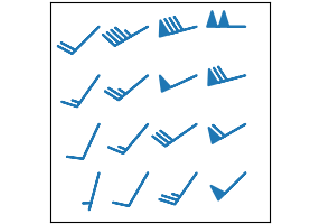
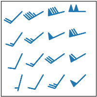
barbs(X, Y, U, V)
https://matplotlib.org/stable/plot_types/arrays/barbs.html
绘制二维风羽图。
参见 barbs。
python
import matplotlib.pyplot as plt
import numpy as np

plt.style.use('_mpl-gallery-nogrid')

# make data:
X, Y = np.meshgrid([1, 2, 3, 4], [1, 2, 3, 4])
angle = np.pi / 180 * np.array([[15., 30, 35, 45],
                                [25., 40, 55, 60],
                                [35., 50, 65, 75],
                                [45., 60, 75, 90]])
amplitude = np.array([[5, 10, 25, 50],
                      [10, 15, 30, 60],
                      [15, 26, 50, 70],
                      [20, 45, 80, 100]])
U = amplitude * np.sin(angle)
V = amplitude * np.cos(angle)

# plot:
fig, ax = plt.subplots()

ax.barbs(X, Y, U, V, barbcolor='C0', flagcolor='C0', length=7, linewidth=1.5)

ax.set(xlim=(0, 4.5), ylim=(0, 4.5))

plt.show()- 下载 Jupyter 笔记本:
barbs.ipynb: https://matplotlib.org/stable/_downloads/b6f78f97f7fbec71abb3c6aefc1d4c7d/barbs.ipynb - 下载 Python 源代码:
barbs.py: https://matplotlib.org/stable/_downloads/417acbb12d2b6a185f7af1ca9b76b6ff/barbs.py - 下载压缩包:
barbs.zip: https://matplotlib.org/stable/_downloads/bd94b7dc54ad2bd65502788388582524/barbs.zip
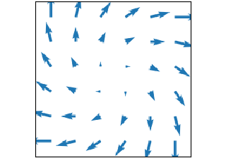
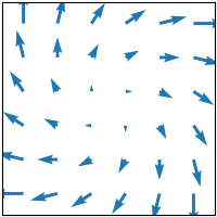
quiver(X, Y, U, V)
https://matplotlib.org/stable/plot_types/arrays/quiver.html
绘制二维箭头场图。
详见 quiver 函数文档。
python
import matplotlib.pyplot as plt
import numpy as np

plt.style.use('_mpl-gallery-nogrid')

# make data
x= np.linspace(-4, 4, 6)
y= np.linspace(-4, 4, 6)
X, Y = np.meshgrid(x, y)
U = x+ Y
V = Y - X

# plot
fig, ax = plt.subplots()

ax.quiver(X, Y, U, V, color="C0", angles='xy',
          scale_units='xy', scale=5, width=.015)

ax.set(xlim=(-5, 5), ylim=(-5, 5))

plt.show()- 下载 Jupyter 笔记本:
quiver.ipynb: https://matplotlib.org/stable/_downloads/27efbe0ba3d7a6ab8f824add7e7bc774/quiver.ipynb - 下载 Python 源代码:
quiver.py: https://matplotlib.org/stable/_downloads/bbc514f3a1016c7b7672428cb8502dbf/quiver.py - 下载压缩包:
quiver.zip: https://matplotlib.org/stable/_downloads/870cc757a73b3a05d4e54928b0d06465/quiver.zip
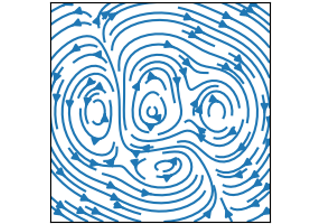
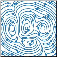
streamplot(X, Y, U, V)
https://matplotlib.org/stable/plot_types/arrays/streamplot.html
绘制向量场的流线图。
详情参阅 streamplot。
python
import matplotlib.pyplot as plt
import numpy as np

plt.style.use('_mpl-gallery-nogrid')

# make a stream function:
X, Y = np.meshgrid(np.linspace(-3, 3, 256), np.linspace(-3, 3, 256))
Z = (1 - X/2 + X**5 + Y**3) * np.exp(-X**2 - Y**2)
# make U and V out of the streamfunction:
V = np.diff(Z[1:, :], axis=1)
U = -np.diff(Z[:, 1:], axis=0)

# plot:
fig, ax = plt.subplots()

ax.streamplot(X[1:, 1:], Y[1:, 1:], U, V)

plt.show()- 下载 Jupyter 笔记本:
streamplot.ipynb: https://matplotlib.org/stable/_downloads/d5495da7bfff8a67e9727dec9dd93ded/streamplot.ipynb - 下载 Python 源代码:
streamplot.py: https://matplotlib.org/stable/_downloads/a00878546a57593e801c23b20668d112/streamplot.py - 下载压缩包:
streamplot.zip: https://matplotlib.org/stable/_downloads/35ebfac96679a1b3a26c0d0d2645d776/streamplot.zip
非规则网格数据
https://matplotlib.org/stable/plot_types/unstructured/index.html
绘制在非结构化网格上的数据\(Z_{x, y})、非结构化坐标网格\((x, y))以及二维函数\(f(x, y) = z)的图表。
tricontour(x, y, z)
tricontourf(x, y, z)
tripcolor(x, y, z)
triplot(x, y)
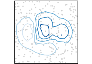
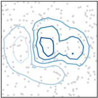
tricontour(x, y, z)
https://matplotlib.org/stable/plot_types/unstructured/tricontour.html
在非结构化三角形网格上绘制等高线。
参见 tricontour。
python
import matplotlib.pyplot as plt
import numpy as np

plt.style.use('_mpl-gallery-nogrid')

# make data:
np.random.seed(1)
x= np.random.uniform(-3, 3, 256)
y= np.random.uniform(-3, 3, 256)
z = (1 - x/2 + x**5 + y**3) * np.exp(-x**2 - y**2)
levels = np.linspace(z.min(), z.max(), 7)

# plot:
fig, ax = plt.subplots()

ax.plot(x, y, 'o', markersize=2, color='lightgrey')
ax.tricontour(x, y, z, levels=levels)

ax.set(xlim=(-3, 3), ylim=(-3, 3))

plt.show()- 下载 Jupyter 笔记本:
tricontour.ipynb: https://matplotlib.org/stable/_downloads/bc15cb912cd995fdd1a278ab73fd7f87/tricontour.ipynb - 下载 Python 源代码:
tricontour.py: https://matplotlib.org/stable/_downloads/940df964c05c80d436d3c80ab81a4fec/tricontour.py - 下载压缩包:
tricontour.zip: https://matplotlib.org/stable/_downloads/bdf1820cd937fd601e353f37118b0d9c/tricontour.zip
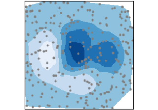
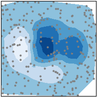
tricontourf(x, y, z)
https://matplotlib.org/stable/plot_types/unstructured/tricontourf.html
在非结构化三角形网格上绘制填充等高线区域。
详情参阅 tricontourf。
python
import matplotlib.pyplot as plt
import numpy as np

plt.style.use('_mpl-gallery-nogrid')

# make data:
np.random.seed(1)
x= np.random.uniform(-3, 3, 256)
y= np.random.uniform(-3, 3, 256)
z = (1 - x/2 + x**5 + y**3) * np.exp(-x**2 - y**2)
levels = np.linspace(z.min(), z.max(), 7)

# plot:
fig, ax = plt.subplots()

ax.plot(x, y, 'o', markersize=2, color='grey')
ax.tricontourf(x, y, z, levels=levels)

ax.set(xlim=(-3, 3), ylim=(-3, 3))

plt.show()- 下载 Jupyter 笔记本:
tricontourf.ipynb: https://matplotlib.org/stable/_downloads/06d8568c9c6f02bf1c64744e15c4a416/tricontourf.ipynb - 下载 Python 源代码:
tricontourf.py: https://matplotlib.org/stable/_downloads/e41d1680a93a490689990af0797a91bd/tricontourf.py - 下载压缩包:
tricontourf.zip: https://matplotlib.org/stable/_downloads/523aaf766630dad5e0af80f4cfffce7f/tricontourf.zip
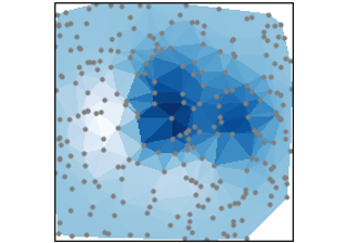
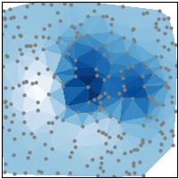
tripcolor(x, y, z)
https://matplotlib.org/stable/plot_types/unstructured/tripcolor.html
创建非结构化三角形网格的伪彩色图。
参见 tripcolor。
python
import matplotlib.pyplot as plt
import numpy as np

plt.style.use('_mpl-gallery-nogrid')

# make data:
np.random.seed(1)
x= np.random.uniform(-3, 3, 256)
y= np.random.uniform(-3, 3, 256)
z = (1 - x/2 + x**5 + y**3) * np.exp(-x**2 - y**2)

# plot:
fig, ax = plt.subplots()

ax.plot(x, y, 'o', markersize=2, color='grey')
ax.tripcolor(x, y, z)

ax.set(xlim=(-3, 3), ylim=(-3, 3))

plt.show()- 下载 Jupyter 笔记本:
tripcolor.ipynb: https://matplotlib.org/stable/_downloads/819e2f1e607e1c86291ce273efb8c565/tripcolor.ipynb - 下载 Python 源代码:
tripcolor.py: https://matplotlib.org/stable/_downloads/4201830e67f8c228b56f01ff0fdd82a4/tripcolor.py - 下载压缩包:
tripcolor.zip: https://matplotlib.org/stable/_downloads/3b6617efe902502d83be9023b7f4ec97/tripcolor.zip
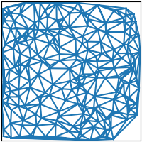
triplot(x, y)
https://matplotlib.org/stable/plot_types/unstructured/triplot.html
绘制非结构化三角网格的线条和/或标记。
详情参阅 triplot。
python
import matplotlib.pyplot as plt
import numpy as np

plt.style.use('_mpl-gallery-nogrid')

# make data:
np.random.seed(1)
x= np.random.uniform(-3, 3, 256)
y= np.random.uniform(-3, 3, 256)
z = (1 - x/2 + x**5 + y**3) * np.exp(-x**2 - y**2)

# plot:
fig, ax = plt.subplots()

ax.triplot(x, y)

ax.set(xlim=(-3, 3), ylim=(-3, 3))

plt.show()- 下载 Jupyter 笔记本:
triplot.ipynb: https://matplotlib.org/stable/_downloads/ca2a498beb12619961d43a7ba14a3ed1/triplot.ipynb - 下载 Python 源代码:
triplot.py: https://matplotlib.org/stable/_downloads/569f6d2696dbae812695e6d633b45b03/triplot.py - 下载压缩包:
triplot.zip: https://matplotlib.org/stable/_downloads/7e879d7f6ffa630b6bf1b6dca964f733/triplot.zip
三维与体积数据可视化
https://matplotlib.org/stable/plot_types/3D/index.html
使用 mpl_toolkits.mplot3d 库绘制三维数据 \((x,y,z))、曲面数据 \(f(x,y)=z) 以及体积数据 \(V_{x, y, z})。
bar3d(x, y, z, dx, dy, dz)
fill_between(x1, y1, z1, x2, y2, z2)
fill_between(x1, y1, z1, x2, y2, z2)
plot(xs, ys, zs)
quiver(X, Y, Z, U, V, W)
scatter(xs, ys, zs)
stem(x, y, z)
plot_surface(X, Y, Z)
plot_trisurf(x, y, z)
voxels(\[x, y, z, filled)](voxels_simple.html#sphx-glr-plot-types-3d-voxels-simple-py)
voxels(x, y, z, filled)
plot_wireframe(X, Y, Z)
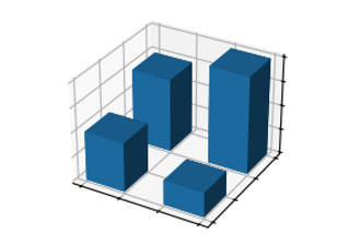
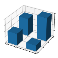
bar3d(x, y, z, dx, dy, dz)
https://matplotlib.org/stable/plot_types/3D/bar3d_simple.html
参见 bar3d。
python
import matplotlib.pyplot as plt
import numpy as np

plt.style.use('_mpl-gallery')

# Make data
x = [1, 1, 2, 2]
y = [1, 2, 1, 2]
z = [0, 0, 0, 0]
dx = np.ones_like(x)*0.5
dy = np.ones_like(x)*0.5
dz = [2, 3, 1, 4]

# Plot
fig, ax = plt.subplots(subplot_kw={"projection": "3d"})
ax.bar3d(x, y, z, dx, dy, dz)

ax.set(xticklabels=[],
       yticklabels=[],
       zticklabels=[])

plt.show()- 下载 Jupyter 笔记本:
bar3d_simple.ipynb: https://matplotlib.org/stable/_downloads/105325b5bfeb925dc4c29468ae7f7a82/bar3d_simple.ipynb - 下载 Python 源代码:
bar3d_simple.py: https://matplotlib.org/stable/_downloads/6dd574408d4e7ff99ff70d35985fd265/bar3d_simple.py - 下载压缩包:
bar3d_simple.zip: https://matplotlib.org/stable/_downloads/484534bf7a851af713d6d3244c93a8aa/bar3d_simple.zip
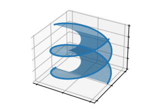
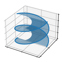
fill_between(x1, y1, z1, x2, y2, z2)
https://matplotlib.org/stable/plot_types/3D/fill_between3d_simple.html
参见 fill_between。
python
import matplotlib.pyplot as plt
import numpy as np

plt.style.use('_mpl-gallery')

# Make data for a double helix
n = 50
theta = np.linspace(0, 2*np.pi, n)
x1 = np.cos(theta)
y1= np.sin(theta)
z1 = np.linspace(0, 1, n)
x2 = np.cos(theta + np.pi)
y2 = np.sin(theta + np.pi)
z2 = z1

# Plot
fig, ax = plt.subplots(subplot_kw={"projection": "3d"})
ax.fill_between(x1, y1, z1, x2, y2, z2, alpha=0.5)
ax.plot(x1, y1, z1, linewidth=2, color='C0')
ax.plot(x2, y2, z2, linewidth=2, color='C0')

ax.set(xticklabels=[],
       yticklabels=[],
       zticklabels=[])

plt.show()- 下载 Jupyter 笔记本:
fill_between3d_simple.ipynb: https://matplotlib.org/stable/_downloads/47197aff0b8ae49d54507a61effbe20c/fill_between3d_simple.ipynb - 下载 Python 源代码:
fill_between3d_simple.py: https://matplotlib.org/stable/_downloads/4b09ece01bb31d76e8210b7150521c3c/fill_between3d_simple.py - 下载压缩包:
fill_between3d_simple.zip: https://matplotlib.org/stable/_downloads/2ac4eceb12f5814b485768cdf6261874/fill_between3d_simple.zip
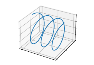
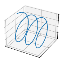
plot(xs, ys, zs)
https://matplotlib.org/stable/plot_types/3D/plot3d_simple.html
参见 plot。
python
import matplotlib.pyplot as plt
import numpy as np

plt.style.use('_mpl-gallery')

# Make data
n = 100
xs = np.linspace(0, 1, n)
ys = np.sin(xs * 6 * np.pi)
zs = np.cos(xs * 6 * np.pi)

# Plot
fig, ax = plt.subplots(subplot_kw={"projection": "3d"})
ax.plot(xs, ys, zs)

ax.set(xticklabels=[],
       yticklabels=[],
       zticklabels=[])

plt.show()- 下载 Jupyter 笔记本:
plot3d_simple.ipynb: https://matplotlib.org/stable/_downloads/9668ea8d423c0e9bc73028daac3c0e8d/plot3d_simple.ipynb - 下载 Python 源代码:
plot3d_simple.py: https://matplotlib.org/stable/_downloads/fa0df995bf922691445c2d10ae27e915/plot3d_simple.py - 下载压缩包:
plot3d_simple.zip: https://matplotlib.org/stable/_downloads/66c973dc08da83f27835405ec48460c0/plot3d_simple.zip
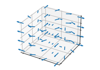
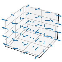
quiver(X, Y, Z, U, V, W)
https://matplotlib.org/stable/plot_types/3D/quiver3d_simple.html
参见 quiver 文档。
python
import matplotlib.pyplot as plt
import numpy as np

plt.style.use('_mpl-gallery')

# Make data
n = 4
x= np.linspace(-1, 1, n)
y= np.linspace(-1, 1, n)
z = np.linspace(-1, 1, n)
X, Y, Z = np.meshgrid(x, y, z)
U = (x+ Y)/5
V = (Y - X)/5
W = Z*0

# Plot
fig, ax = plt.subplots(subplot_kw={"projection": "3d"})
ax.quiver(X, Y, Z, U, V, W)

ax.set(xticklabels=[],
       yticklabels=[],
       zticklabels=[])

plt.show()- 下载 Jupyter 笔记本:
quiver3d_simple.ipynb: https://matplotlib.org/stable/_downloads/96d4baccdd2be2fa187e219d4e203258/quiver3d_simple.ipynb - 下载 Python 源代码:
quiver3d_simple.py: https://matplotlib.org/stable/_downloads/bacb0e8985efda3d3a8ee00460ed06c3/quiver3d_simple.py - 下载压缩包:
quiver3d_simple.zip: https://matplotlib.org/stable/_downloads/2d9fe906fc75014b66a5eeeaa8e8e876/quiver3d_simple.zip
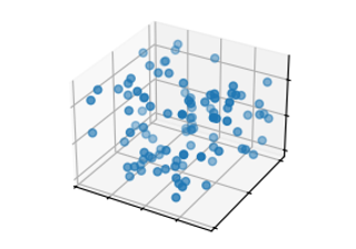
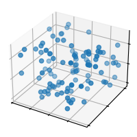
scatter(xs, ys, zs)
https://matplotlib.org/stable/plot_types/3D/scatter3d_simple.html
参见 scatter 文档。
python
import matplotlib.pyplot as plt
import numpy as np

plt.style.use('_mpl-gallery')

# Make data
np.random.seed(19680801)
n = 100
rng = np.random.default_rng()
xs = rng.uniform(23, 32, n)
ys = rng.uniform(0, 100, n)
zs = rng.uniform(-50, -25, n)

# Plot
fig, ax = plt.subplots(subplot_kw={"projection": "3d"})
ax.scatter(xs, ys, zs)

ax.set(xticklabels=[],
       yticklabels=[],
       zticklabels=[])

plt.show()- 下载 Jupyter 笔记本:
scatter3d_simple.ipynb: https://matplotlib.org/stable/_downloads/6456ec22210b5ac17dfa7e88c007d7fc/scatter3d_simple.ipynb - 下载 Python 源代码:
scatter3d_simple.py: https://matplotlib.org/stable/_downloads/7ace3c2232efcb0fd94e4999de5d1b3d/scatter3d_simple.py - 下载压缩包:
scatter3d_simple.zip: https://matplotlib.org/stable/_downloads/03688ffb75eaa3d3d0993b54c34ec69c/scatter3d_simple.zip
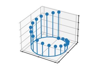
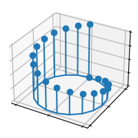
stem(x, y, z)
https://matplotlib.org/stable/plot_types/3D/stem3d.html
参见 stem。
python
import matplotlib.pyplot as plt
import numpy as np

plt.style.use('_mpl-gallery')

# Make data
n = 20
x= np.sin(np.linspace(0, 2*np.pi, n))
y= np.cos(np.linspace(0, 2*np.pi, n))
z = np.linspace(0, 1, n)

# Plot
fig, ax = plt.subplots(subplot_kw={"projection": "3d"})
ax.stem(x, y, z)

ax.set(xticklabels=[],
       yticklabels=[],
       zticklabels=[])

plt.show()- 下载 Jupyter 笔记本:
stem3d.ipynb: https://matplotlib.org/stable/_downloads/cabc7543d4fe87236fdb8bb878823cd2/stem3d.ipynb - 下载 Python 源代码:
stem3d.py: https://matplotlib.org/stable/_downloads/7236513de029a7bc6ac29aed9db1bf91/stem3d.py - 下载压缩包:
stem3d.zip: https://matplotlib.org/stable/_downloads/a5f6454f7df0e8de030ce37580117307/stem3d.zip
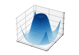
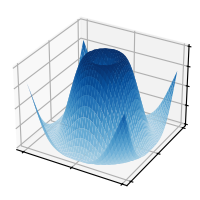
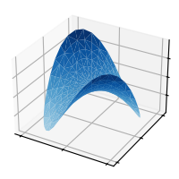
plot_surface(X, Y, Z)
https://matplotlib.org/stable/plot_types/3D/surface3d_simple.html
参见 plot_surface。
python
import matplotlib.pyplot as plt
import numpy as np

from matplotlib import cm

plt.style.use('_mpl-gallery')

# Make data
x= np.arange(-5, 5, 0.25)
Y = np.arange(-5, 5, 0.25)
X, Y = np.meshgrid(X, Y)
R = np.sqrt(X**2 + Y**2)
Z = np.sin(R)

# Plot the surface
fig, ax = plt.subplots(subplot_kw={"projection": "3d"})
ax.plot_surface(X, Y, Z, vmin=Z.min() * 2, cmap=cm.Blues)

ax.set(xticklabels=[],
       yticklabels=[],
       zticklabels=[])

plt.show()- 下载 Jupyter 笔记本:
surface3d_simple.ipynb: https://matplotlib.org/stable/_downloads/2fbb51497dcb6c194a7be35176511d73/surface3d_simple.ipynb - 下载 Python 源代码:
surface3d_simple.py: https://matplotlib.org/stable/_downloads/0c69e8950c767c2d95108979a24ace2f/surface3d_simple.py - 下载压缩包:
surface3d_simple.zip: https://matplotlib.org/stable/_downloads/1fcd655f21c26798cc10fe85926d2fc7/surface3d_simple.zip
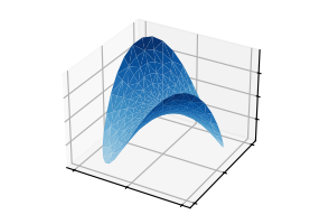
plot_trisurf(x, y, z)
https://matplotlib.org/stable/plot_types/3D/trisurf3d_simple.html
参见 plot_trisurf。
python
import matplotlib.pyplot as plt
import numpy as np

from matplotlib import cm

plt.style.use('_mpl-gallery')

n_radii = 8
n_angles = 36

# Make radii and angles spaces
radii = np.linspace(0.125, 1.0,n_radii)
angles = np.linspace(0, 2*np.pi, n_angles, endpoint=False)[..., np.newaxis]

# Convert polar (radii, angles) coords to cartesian (x, y) coords.
x= np.append(0, (radii*np.cos(angles)).flatten())
y= np.append(0, (radii*np.sin(angles)).flatten())
z = np.sin(-x*y)

# Plot
fig, ax = plt.subplots(subplot_kw={'projection': '3d'})
ax.plot_trisurf(x, y, z, vmin=z.min() * 2, cmap=cm.Blues)

ax.set(xticklabels=[],
       yticklabels=[],
       zticklabels=[])

plt.show()- 下载 Jupyter 笔记本:
trisurf3d_simple.ipynb: https://matplotlib.org/stable/_downloads/cd674f07796f1263c2618071b6eb1746/trisurf3d_simple.ipynb - 下载 Python 源代码:
trisurf3d_simple.py: https://matplotlib.org/stable/_downloads/e3e638c790e8cedaa78c03303fd6f563/trisurf3d_simple.py - 下载压缩包:
trisurf3d_simple.zip: https://matplotlib.org/stable/_downloads/feaa60e57c5df8addf5e8058d10efe16/trisurf3d_simple.zip
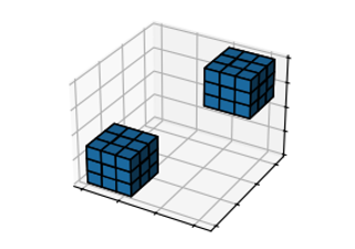
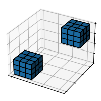
voxels(x, y, z, filled)
https://matplotlib.org/stable/plot_types/3D/voxels_simple.html
参见 voxels 文档。
python
import matplotlib.pyplot as plt
import numpy as np

plt.style.use('_mpl-gallery')

# Prepare some coordinates
x, y, z = np.indices((8, 8, 8))

# Draw cuboids in the top left and bottom right corners
cube1 = (x< 3) & (y< 3) & (z < 3)
cube2 = (x>= 5) & (y>= 5) & (z >= 5)

# Combine the objects into a single boolean array
voxelarray = cube1 | cube2

# Plot
fig, ax = plt.subplots(subplot_kw={"projection": "3d"})
ax.voxels(voxelarray, edgecolor='k')

ax.set(xticklabels=[],
       yticklabels=[],
       zticklabels=[])

plt.show()- 下载 Jupyter 笔记本:
voxels_simple.ipynb: https://matplotlib.org/stable/_downloads/4fc11b0e276d5ef6db9f31bfbba6c141/voxels_simple.ipynb - 下载 Python 源代码:
voxels_simple.py: https://matplotlib.org/stable/_downloads/88852f40d7e531f3d8efe9db69d12d9c/voxels_simple.py - 下载压缩包:
voxels_simple.zip: https://matplotlib.org/stable/_downloads/199ca7c26dbfe5a62f3085fdb3823a77/voxels_simple.zip
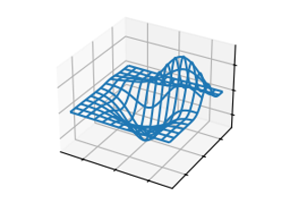
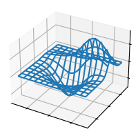
plot_wireframe(X, Y, Z)
https://matplotlib.org/stable/plot_types/3D/wire3d_simple.html
参见 plot_wireframe。
python
import matplotlib.pyplot as plt

from mpl_toolkits.mplot3d import axes3d

plt.style.use('_mpl-gallery')

# Make data
X, Y, Z = axes3d.get_test_data(0.05)

# Plot
fig, ax = plt.subplots(subplot_kw={"projection": "3d"})
ax.plot_wireframe(X, Y, Z, rstride=10, cstride=10)

ax.set(xticklabels=[],
       yticklabels=[],
       zticklabels=[])

plt.show()- 下载 Jupyter 笔记本:
wire3d_simple.ipynb: https://matplotlib.org/stable/_downloads/c14ff0fa876858aa18b6c08cfc360aa5/wire3d_simple.ipynb - 下载 Python 源代码:
wire3d_simple.py: https://matplotlib.org/stable/_downloads/3fc633415467280d09654ac462420fdd/wire3d_simple.py - 下载压缩包:
wire3d_simple.zip: https://matplotlib.org/stable/_downloads/d1248584d9ef37a5c5d3b050e8ac35c5/wire3d_simple.zip
2025-09-10(三)