目录
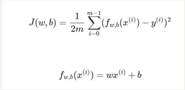
成本函数以及目标预测函数
# y-hat 目标值预测函数
def compute_model_output(x, w, b):
"""
Computes the prediction of a linear model
Args:
x (ndarray (m,)): Data, m examples
w,b (scalar) : model parameters
Returns
y (ndarray (m,)): target values
"""
m = x.shape[0]
# m=len(x)
f_wb = np.zeros(m)
for i in range(m):
f_wb[i] = w * x[i] + b
return f_wb
# 成本函数计算
def compute_cost(x, y, w, b):
"""
Computes the cost function for linear regression.
Args:
x (ndarray (m,)): Data, m examples
y (ndarray (m,)): target values
w,b (scalar) : model parameters
Returns
total_cost (float): The cost of using w,b as the parameters for linear regression
to fit the data points in x and y
"""
# number of training examples
m = x.shape[0]
cost_sum = 0
for i in range(m):
f_wb = w * x[i] + b
cost = (f_wb - y[i]) ** 2
cost_sum = cost_sum + cost
total_cost = (1 / (2 * m)) * cost_sum
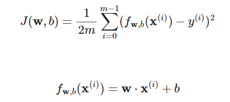
return total_costJ(w,b)是成本函数,f(w,b)是预测函数
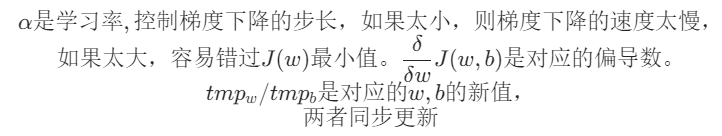
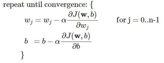
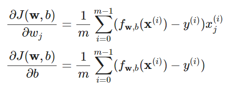
梯度下降函数
python
def compute_gradient(x, y, w, b):
    """
    Computes the gradient for linear regression
    Args:
      x (ndarray (m,)): Data, m examples
      y (ndarray (m,)): target values
      w,b (scalar)    : model parameters
    Returns
      dj_dw (scalar): The gradient of the cost w.r.t. the parameters w
      dj_db (scalar): The gradient of the cost w.r.t. the parameter b
     """

    # Number of training examples
    m = x.shape[0]
    dj_dw = 0
    dj_db = 0

    for i in range(m):
        f_wb = w * x[i] + b
        dj_dw_i = (f_wb - y[i]) * x[i]
        dj_db_i = f_wb - y[i]
        dj_db += dj_db_i
        dj_dw += dj_dw_i
    dj_dw = dj_dw / m
    dj_db = dj_db / m

    return dj_dw, dj_db
线性回归的梯度下降
注意:当成本函数是一个凸函数(碗)时,使用梯度下降模型可以找到成本函数最小值,但是如果不是一个凸函数,从某一个初始值出发,只能找到成本函数局部最小值
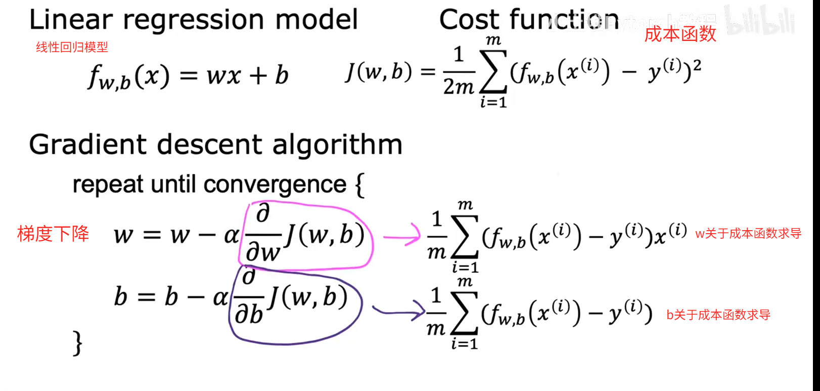
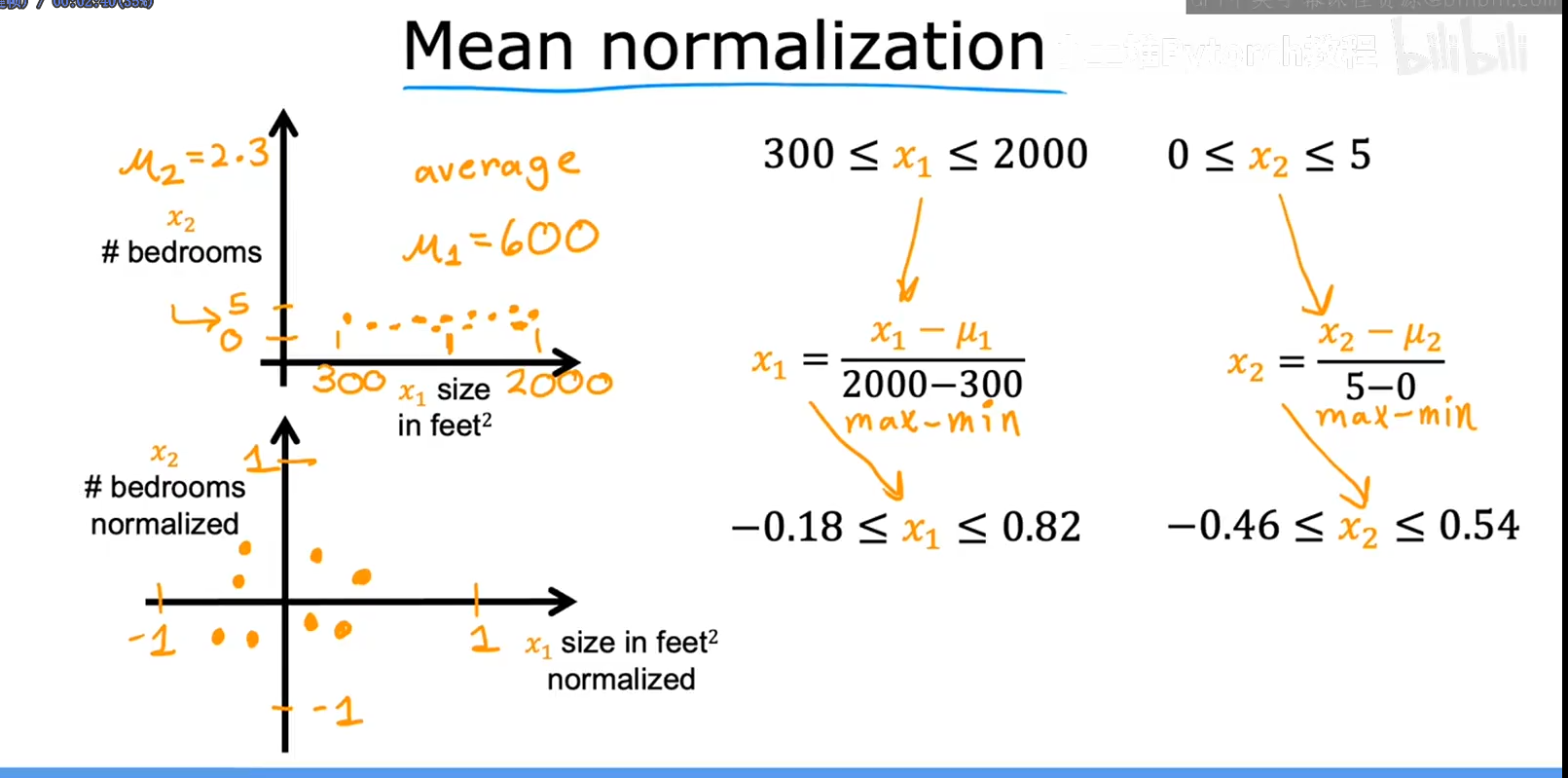
特征缩放
均值归一化
- 找到训练集上的均值
- 按照以下公式进行计算
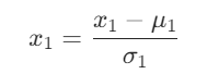
Z分数归一化
- 找到训练集上的均值
,计算得到每个特征值的标准差
- 按照以下公式进行计算

python
def zscore_normalize_features(X):
    mu = np.mean(X, axis=0) # 求均值
    sigma = np.std(X, axis=0)# 求标准差
    X_norm = (X - mu) / sigma
    return X_norm
多特征线性回归
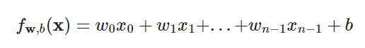
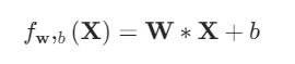
预测函数
成本函数
梯度下降函数
公式实现
代码实现
python
import copy, math
import numpy as np
import matplotlib.pyplot as plt
plt.style.use('./deeplearning.mplstyle')
np.set_printoptions(precision=2) # reduced display precision on numpy arrays
X_train = np.array([[2104,5,1,45],[1416,3,2,40],[852,2,1,35]])
y_train = np.array([460,232,178])
b_init = 785.1811367994083
w_init = np.array([ 0.39133535, 18.75376741, -53.36032453, -26.42131618])
# 接下来实现成本函数J(w,b)
def computer_cost(x,y,w,b):
m = x.shape[0]
cost = 0.0
for i in range(m):
f_wb_i = np.dot(x[i],w)+b
cost = cost + (f_wb_i-y[i])**2
cost = cost/(2*m)
return cost
# 接下来实现求偏导函数
def computer_gradient(x,y,w,b):
m,n = x.shape
dj_dw = np.zeros((n,))
dj_db = 0.
for i in range(m):
err = (np.dot(x[i], w) + b) - y[i]
for j in range(n):
dj_dw[j] = dj_dw[j] + err * x[i, j]
dj_db = dj_db + err
dj_dw = dj_dw / m
dj_db = dj_db / m
return dj_dw, dj_db
# 接下来实现梯度下降函数
def gradient_descent(x, y, w_in, b_in, cost_function, gradient_function, alpha, num_iters):
J_history = []
w = copy.deepcopy(w_in) # avoid modifying global w within function
b = b_in
for i in range(num_iters):
dj_dw,dj_db= gradient_function(x, y, w, b) # 计算偏导
w = w - alpha * dj_dw
b = b - alpha * dj_db
# 保存每个成本函数值,用于观测成本函数的下降
if i < 100000: # prevent resource exhaustion
J_history.append(cost_function(x, y, w, b))
# Print cost every at intervals 10 times or as many iterations if < 10
if i % math.ceil(num_iters / 10) == 0:
print(f"Iteration {i:4d}: Cost {J_history[-1]:8.2f} ")
return w, b, J_history # return final w,b and J history for graphing
init_w = np.zeros_like(w_init)
init_b = 0
num_iters = 10000
alpha = 5.0e-7
w_final,b_final,J_hist = gradient_descent(X_train,y_train,init_w,init_b,computer_cost,computer_gradient,alpha,num_iters)
print(f"b,w found by gradient descent: {b_final:0.2f},{w_final} ")
m,_ = X_train.shape
for i in range(m):
print(f"prediction: {np.dot(X_train[i], w_final) + b_final:0.2f}, target value: {y_train[i]}")
# plot cost versus iteration
fig, (ax1, ax2) = plt.subplots(1, 2, constrained_layout=True, figsize=(12, 4))
ax1.plot(J_hist)
ax2.plot(100 + np.arange(len(J_hist[100:])), J_hist[100:])
ax1.set_title("Cost vs. iteration"); ax2.set_title("Cost vs. iteration (tail)")
ax1.set_ylabel('Cost') ; ax2.set_ylabel('Cost')
ax1.set_xlabel('iteration step') ; ax2.set_xlabel('iteration step')
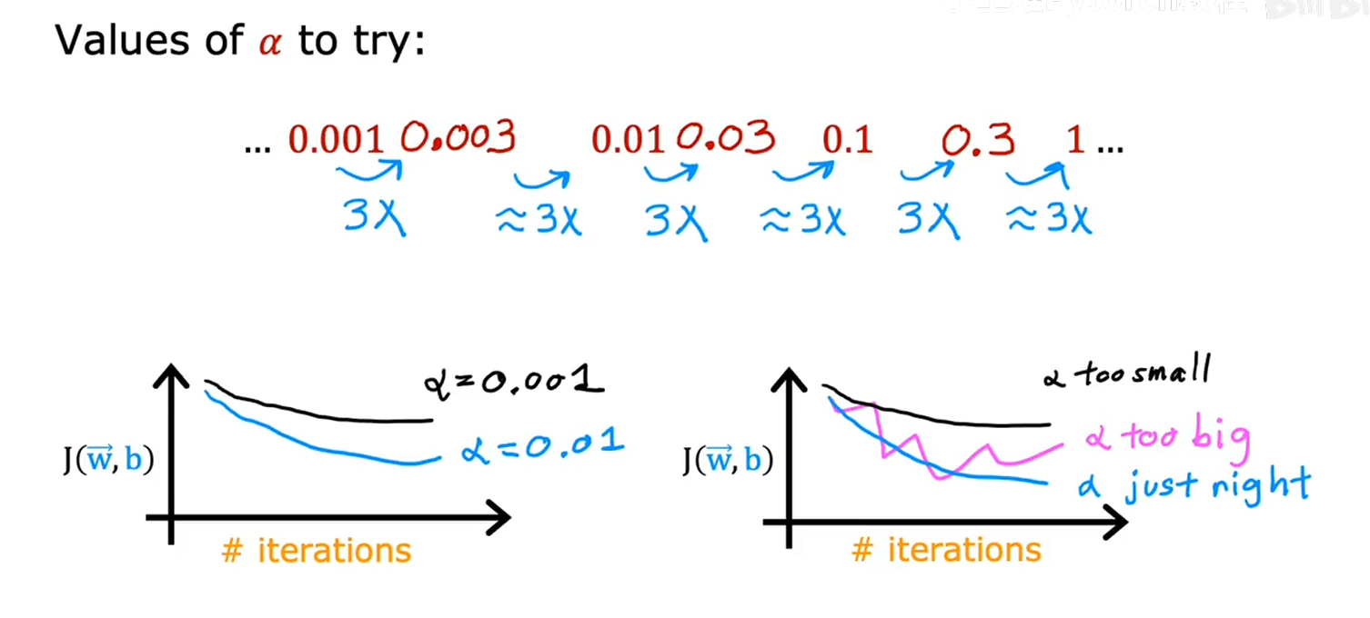
plt.show()如何选择合适学习率
学习曲线可能出现以下的几种情况
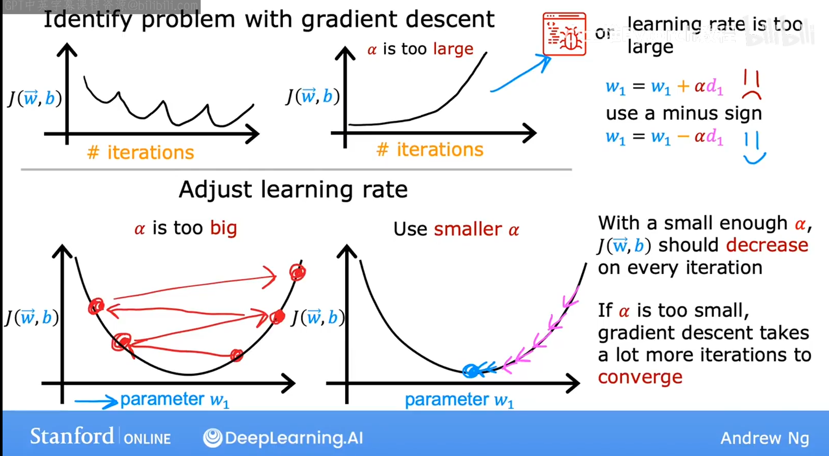
进行学习率选择时候,可以先设置一个很小的学习率,使得成本函数下降很慢,或者选择一个很大的学习率,使得成本函数下降不规矩,最后找到一个合适的学习率
特征工程
根据问题的实际情况,进行新特征的设计,就是特征工程,利用对问题的理解或者直觉来设计新特征,通常是通过改造或组合问题的原有特征,以便让更容易的让学习算法做出准确的预测。
多项式回归
相比较于单项式回归,多项式回归将可选特性提升到了二次方、三次方或者更高,与此同时,特征缩放就变得更加重要
SKlearn的使用
基本使用代码
python
import numpy as np
np.set_printoptions(precision=2)
from sklearn.linear_model import LinearRegression, SGDRegressor
from sklearn.preprocessing import StandardScaler
from lab_utils_multi import  load_house_data
import matplotlib.pyplot as plt
dlblue = '#0096ff'; dlorange = '#FF9300'; dldarkred='#C00000'; dlmagenta='#FF40FF'; dlpurple='#7030A0';
plt.style.use('./deeplearning.mplstyle')


# 加载数据进行特征缩放
X_train, y_train = load_house_data()
X_features = ['size(sqft)','bedrooms','floors','age']

scaler = StandardScaler()
X_norm = scaler.fit_transform(X_train)
print(f"Peak to Peak range by column in Raw     X:{np.ptp(X_train,axis=0)}")
print(f"Peak to Peak range by column in Normalized X:{np.ptp(X_norm,axis=0)}")

# 创建并拟合回归模型
sgdr = SGDRegressor(max_iter=1000)
sgdr.fit(X_norm, y_train) # 进行了拟合

print(sgdr)
print(f"number of iterations completed: {sgdr.n_iter_}, number of weight updates: {sgdr.t_}")

b_norm = sgdr.intercept_
w_norm = sgdr.coef_
print(f"model parameters:w: {w_norm}, b:{b_norm}")

# 进行预测
# make a prediction using sgdr.predict()
y_pred_sgd = sgdr.predict(X_norm)
# make a prediction using w,b.
y_pred = np.dot(X_norm, w_norm) + b_norm
# 两种方式的到的预测值相同
print(f"Prediction on training set:\n{y_pred[:4]}" )
print(f"Target values \n{y_train[:4]}")

# 通过图像绘制,比较目标值和预测值
fig,ax=plt.subplots(1,4,figsize=(12,3),sharey=True)
for i in range(len(ax)):
    ax[i].scatter(X_train[:,i],y_train, label = 'target')
    ax[i].set_xlabel(X_features[i])
    ax[i].scatter(X_train[:,i],y_pred,color=dlorange, label = 'predict')
ax[0].set_ylabel("Price"); ax[0].legend();
fig.suptitle("target versus prediction using z-score normalized model")
plt.show()
Scikit-learn 框架中有一个梯度下降回归模型,名为 sklearn.linear_model.SGDRegressor.
sklearn.preprocessing.StandardScaler 将按照之前实验中的方式执行 z 分数标准化操作。在这里,它被称为"standard score"。
关键函数
- Z-分数归一化函数
python
scaler = StandardScaler()
X_norm = scaler.fit_transform(X_train)- 梯度下降函数
python
sgdr = SGDRegressor(max_iter=1000) # 梯度下降函数
sgdr.fit(X_norm, y_train) # 拟合函数- 预测函数
python
y_pred_sgd = sgdr.predict(X_norm)- 成本函数:成本函数的计算包含在了SGDRegressor中,不需要再额外计算