Title
题目
Acquisition-independent deep learning for quantitative MRI parameter estimation using neural controlled differential equations
基于神经控制微分方程的采集无关深度学习用于定量MRI参数估计
01
文献速递介绍
定量磁共振成像(QMRI)参数作为影像生物标志物的应用及神经控制微分方程(NCDEs)的突破 定量磁共振成像(QMRI)参数等影像生物标志物,是辅助多种病变的病灶检测、定性分析及治疗监测的便捷、经济、可重复且无创的工具,有助于改善患者诊疗质量。QMRI技术可生成用于评估组织形态、生物学特征及功能的参数,其已证实的临床实用场景包括肿瘤监测(Chauvie等,2023;O'Connor等,2017)、脑卒中成像(Albers,1998)、心肌异常检测(Manfrini等,2021;Taylor等,2016)以及铁过载检测(Liden等,2021)。目前研究较多的QMRI技术包括:用于弥散加权成像(DWI)的体素内不相干运动(IVIM MRI)模型、基于可变翻转角的T1弛豫测量(VFA T1映射),以及动态对比增强磁共振成像(DCE-MRI)。 在QMRI中,组织特性需通过一系列MRI数据,结合生物物理模型进行估计------该模型通过QMRI参数将测得的MRI信号与潜在组织特性关联起来。传统上,此类参数通过最小二乘拟合(LSQ)方法估计,从具有不同对比度权重的MR图像中提取QMRI参数。最小二乘拟合是一种迭代过程,旨在最小化观测MRI数据与重建信号曲线之间的平方差之和。尽管在信噪比(SNR)较高时,最小二乘拟合是生理参数的可靠估计方法,但它仍存在显著局限性:当信噪比偏低时,忽略空间信息、信号曲线噪声干扰以及非凸目标函数的综合作用,会导致QMRI参数估计结果的方差显著增大(Barbieri等,2016;Neil与Bretthorst,1993;While,2017)。参数估计的重复性与准确性受损,已成为QMRI技术临床应用的关键障碍(Kurland等,2012;Rosenkrantz等,2015)。 近年来的研究表明,具有非线性映射学习能力的深度学习,可作为多种QMRI模型参数估计中最小二乘拟合的有效替代方案。尤其在提升估计准确性与精确度、加快参数估计速度,以及减少患者参数测量的日间波动方面,深度学习展现出明显优势(Barbieri等,2020;Bliesener等,2020;Gurney-Champion等,2022;Kaandorp等,2021;Ottens等,2022;Ulas等,2019)。然而,与最小二乘拟合不同,现有深度学习方法对不同磁共振采集协议的鲁棒性不足:这类方法的输入依赖固定集合的输入信号(如全连接网络(Bliesener等,2020;Kaandorp等,2021;Ulas等,2019)与卷积网络(Huang,2022;Vasylechko等,2022)),或规则采样的信号序列(如循环神经网络(Ottens等,2022))。在实际应用中,不同研究与临床场景下的QMRI采集协议差异显著(Ljimani等,2020),且采集设置通常不遵循等距采样模式(例如翻转角为2°、5°、10°、25°)。因此,当前深度学习方法可视为"特定于采集协议"的方法------即尽管模型架构可复用,但每种采集协议都需对应一个专用模型,并配备专用训练数据及相应的训练与验证流程。现有QMRI参数估计深度学习方法在泛化性与实用性上的欠缺,阻碍了这类算法在临床试验及临床实践中的推广。特别是,对"特定于采集协议模型"的需求意味着,每次调整扫描仪设置都需单独进行训练与验证,这不仅增加了流程复杂性,还可能导致不同协议下的结果不一致。因此,一种"与采集协议无关"的方法,对于将深度学习融入QMRI参数估计的临床工作流程至关重要。 与此同时,一类名为"神经常微分方程"的机器学习方法得以发展,其通过训练神经网络学习潜在微分方程,实现对连续时间系统动态的近似(Chen,2018)。神经控制微分方程(NCDEs)在该框架基础上进一步拓展:通过整合输入数据,利用观测结果控制已学习的微分方程,从而使输出与已学习的系统动态及输入序列形成明确关联(Kidger,2020)。NCDEs通过三次样条将离散输入转换为连续平滑的轨迹,能够处理不规则、不完整且长度可变的数据,进而通过控制微分方程对隐藏状态的演化进行建模。这一特性使NCDEs成为QMRI参数估计的极具潜力的方法。 本研究假设,NCDEs可作为通用的、与采集协议无关的网络,用于QMRI参数估计。这一方法有望解决上述现有技术的缺陷,为将深度学习融入QMRI临床工作流程铺平道路。 本研究的主要贡献如下: - 通过将NCDEs应用于QMRI参数估计,克服了神经网络"特定于磁共振采集协议"的局限性。 - 在模拟数据上验证了NCDEs在VFA T1映射、IVIM MRI及扩展Tofts-Kety模型DCE-MRI中的性能。 - 在在体数据上验证了NCDEs在VFA T1映射与IVIM MRI中的性能。 - 实验结果表明,无论在模拟实验还是在体实验中,NCDEs在QMRI参数估计方面均优于传统最小二乘拟合。 - 实验结果表明,无论在模拟实验还是在体实验中,NCDEs与"特定于采集协议"的多层感知器在QMRI参数估计性能上相当。
Aastract
摘要
Deep learning has proven to be a suitable alternative to least squares (LSQ) fitting for parameter estimation in various quantitative MRI (QMRI) models. However, current deep learning implementations are not robust to changes in MR acquisition protocols. In practice, QMRI acquisition protocols differ substantially between different studies and clinical settings. The lack of generalizability and adoptability of current deep learning approaches for QMRI parameter estimation impedes the implementation of these algorithms in clinical trials and clinical practice. Neural Controlled Differential Equations (NCDEs) allow for the sampling of incomplete and irregularly sampled data with variable length, making them ideal for use in QMRI parameter estimation. In this study, we show that NCDEs can function as a generic tool for the accurate estimation of QMRI parameters, regardless of QMRI sequence length, configuration of independent variables and QMRI forward model (variable flip angle T1-mapping, intravoxel incoherent motion MRI, dynamic contrast-enhanced MRI). NCDEs achieved lower mean squared error than LSQ fitting in low-SNR simulations and in vivo in challenging anatomical regions like the abdomen and leg, but this improvement was no longer evident at high SNR. When NCDEs improve parameter estimation, they tend to do so by reducing the variance in estimation errors. These findings suggest that NCDEs offer a robust approach for reliable QMRI parameter estimation, especially in scenarios with high uncertainty or low image quality. We believe that with NCDEs, we have solved one of the main challenges for using deep learning for QMRI parameter estimation in a broader clinical and research setting
深度学习在定量磁共振成像(QMRI)参数估计中的应用与神经控制微分方程(NCDEs)的优势 在各类定量磁共振成像(QMRI)模型的参数估计任务中,深度学习已被证实是最小二乘(LSQ)拟合的有效替代方案。然而,当前深度学习方法的性能易受磁共振(MR)采集协议变化的影响,鲁棒性不足。在实际应用中,不同研究及临床场景下的QMRI采集协议差异显著。现有QMRI参数估计深度学习方法在泛化性与实用性上的欠缺,阻碍了这类算法在临床试验及临床实践中的推广落地。 神经控制微分方程(NCDEs)能够对长度可变的不完整、非规则采样数据进行处理,这一特性使其成为QMRI参数估计的理想工具。本研究表明,无论QMRI序列长度、自变量配置及QMRI正向模型(可变翻转角T1映射、体素内不相干运动MRI、动态对比增强MRI)如何,NCDEs均可作为一种通用工具,实现QMRI参数的精准估计。 在低信噪比(SNR)模拟实验及腹部、腿部等解剖结构复杂的在体实验中,NCDEs的均方误差(MSE)低于LSQ拟合;但在高信噪比场景下,这种优势不再显著。当NCDEs提升参数估计性能时,其主要通过降低估计误差的方差来实现。这些结果表明,NCDEs为可靠的QMRI参数估计提供了一种鲁棒性方法,尤其适用于不确定性高或图像质量低的场景。我们认为,借助NCDEs,我们已解决了在更广泛的临床与研究场景中,将深度学习应用于QMRI参数估计所面临的主要挑战之一。
Method
方法
All analyses were performed using Python (v3.8, Python Software Foundation) and PyTorch (v1.13.1, PyTorch Foundation). Our code is available at: https://github.com/DKuppens/NCDE-QMRI.
2.1. Quantitative MRI
QMRI models allow us to assess tissue properties by using biophysical models to describe the MRI signal intensity as a function of a changing independent variable, such as flip angle (FA) in VFA T1- mapping, diffusion weighting (b-value) in IVIM MRI and time (t) in DCEMRI.In VFA T1-mapping, the longitudinal spin relaxation time (T1) is estimated by acquiring multiple spoiled gradient-echo readouts, each with different excitation flip angles (FA). Consequently, the signal (s) at FA* depends on T1, the repetition time (TR), and the magnetization at thermal equilibrium (s0) (Christensen, 1974; Gupta, 1977): s(FA, TR) = s01 − exp( − TR T1 )1 − cos(FA) exp( − TR T1 ) sin(FA) (1)In IVIM MRI, diffusion-weighted gradients are used to sensitize the MRI signal to incoherent motion. By varying the strength and duration of the diffusion-weighted gradients, we are able to separate the effect of incoherent motion from diffusion with a bi-exponential model where the signal (s) intensity at diffusion weighting (b) depends on the diffusion coefficient (D), which indicates tissue cell density and structural integrity, the pseudo-diffusion coefficient (D) and perfusion fraction (f), which reflect tissue vascularization and perfusion, and the baseline signal intensity (s0): s(b) = s0((1 − f) exp( − bD) + f exp( − bD* )). (2) In DCE-MRI, tissue T1 is measured over time after bolus administration of a contrast agent, gadolinium. Gadolinium shortens the tissue T1, allowing the tissue gadolinium concentration over time to be estimated. In turn, the pharmacokinetics of gadolinium reflect the tissue perfusion and blood vessel permeability (Khalifa et al., 2014; Sourbron and Buckley, 2013). In the extended Tofts-Kety Model for DCE-MRI, tissue gadolinium concentration (Ct) at time t depends on the reflux rate (ke), fractional volume of extravascular extracellular space (ve), fractional volume of plasma (vp) and the concentration of gadolinium in blood plasma (Cp) (Kety, 1951; Tofts, 1999): Ct( t, Cp) = vpCp(t) + keve∫t0Cp(τ) exp( − ke(t − τ))dτ. (3) For consistency between QMRI forward models throughout the text, we will refer to Ct as s. For the extended Tofts-Kety DCE-MRI model, we utilized the implementation and fitting routines from the Python package OG_MO_AUMC_ICR_RMH_NL_UK (Orton et al., 2008), available on the OSIPI GitHub repository (van Houdt et al., 2023). In all described experiments, Cp remained fixed and was equal to the version used in (Rata et al., 2015) (for detailed information, see Table S4)..
所有分析均使用Python(3.8版本,Python软件基金会)和PyTorch(1.13.1版本,PyTorch基金会)完成。相关代码可在以下链接获取:https://github.com/DKuppens/NCDE-QMRI。 ## 2.1 定量磁共振成像(QMRI) QMRI模型通过生物物理模型将MRI信号强度描述为独立变量(如可变翻转角T1映射中的翻转角(FA)、体素内不相干运动MRI(IVIM MRI)中的弥散权重(b值)、动态对比增强MRI(DCE-MRI)中的时间(t))的函数,从而实现对组织特性的评估。 在可变翻转角T1映射(VFA T1-mapping) 中,纵向自旋弛豫时间(T1)通过采集多个扰相梯度回波信号来估计,每个信号对应不同的激发翻转角(FA)。因此,翻转角为FA时的信号(s)取决于T1、重复时间(TR)以及热平衡状态下的磁化强度(s₀)(Christensen,1974;Gupta,1977),公式如下: s(FA, TR) = s_0 \\frac{1 - \\exp\\left(-\\frac{TR}{T_1}\\right)}{1 - \\cos(FA) \\exp\\left(-\\frac{TR}{T_1}\\right)} \\sin(FA) (1) 在体素内不相干运动MRI(IVIM MRI) 中,通过弥散加权梯度使MRI信号对不相干运动敏感。通过改变弥散加权梯度的强度和持续时间,可利用双指数模型将不相干运动与弥散效应分离:弥散权重为b值时的信号(s)取决于弥散系数(D,反映组织细胞密度与结构完整性)、伪弥散系数(D)、灌注分数(f,反映组织血管化程度与灌注情况)以及基线信号强度(s₀),公式如下: s(b) = s_0\\left\[(1 - f)\\exp(-bD) + f\\exp(-bD\^)\\right\] (2) 在动态对比增强MRI(DCE-MRI) 中,通过静脉团注对比剂钆(gadolinium)后,随时间测量组织的T1值。钆可缩短组织T1,据此可估计组织内钆浓度随时间的变化;而钆的药代动力学特征又可反映组织灌注情况与血管通透性(Khalifa等,2014;Sourbron与Buckley,2013)。在DCE-MRI的扩展Tofts-Kety模型中,时间t时的组织钆浓度(Cₜ)取决于回流速率(kₑ)、血管外细胞外间隙体积分数(vₑ)、血浆体积分数(vₚ)以及血浆中钆浓度(Cₚ)(Kety,1951;Tofts,1999),公式如下: C_t(t, C_p) = v_p C_p(t) + k_e v_e \\int_0\^t C_p(\\tau) \\exp\\left(-k_e(t - \\tau)\\right)d\\tau (3) 为保证全文中QMRI正向模型的一致性,本文将Cₜ统一记为s。对于扩展Tofts-Kety DCE-MRI模型,我们采用Python包OG_MO_AUMC_ICR_RMH_NL_UK(Orton等,2008)中的实现与拟合程序,该包可在OSIPI的GitHub仓库(van Houdt等,2023)中获取。在所有所述实验中,Cₚ保持固定,其取值与(Rata等,2015)中使用的版本一致(详细信息见表S4)。
Conclusion
结论
NCDEs can function as a generic tool for accurate estimation of quantitative MRI parameters, irrespective of sequence length or quantitative MRI forward model. Overcoming these two hurdles opens up the use of neural networks for quantitative MRI parameter estimation to a broad audience of researchers and clinicians.
神经控制微分方程(NCDEs)可作为一种通用工具,实现定量磁共振成像(QMRI)参数的精准估计,且不受序列长度或QMRI正向模型的限制。攻克这两大难题后,神经网络在QMRI参数估计中的应用范围得以拓展,能惠及更广泛的研究人员与临床医生群体。
Results
结果
3.1. Simulations
3.1.1. VFA T1-mapping
Across all SNR levels < 200, NCDE-based parameter estimation consistently had a lower mean squared error, lower median (except for SNR = 150) and lower 75th percentile of the squared error than LSQ fitting at estimating the relaxation constant T1 (Fig. 2, left). However, at the highest SNR levels (SNR ≥ 200), LSQ fitting performed better than NCDE-based parameter estimation in estimating T1. Both NCDEs and LSQ fitting had more accurate estimates when the input sequence became longer (Fig. 2, center). For all sequence lengths, NCDEs had a lower mean squared error than LSQ fitting in estimating the relaxation constant T1. When evaluated at a fixed acquisition scheme, both NCDEs and MLPs had a lower mean squared error than LSQ fitting at all SNR ≤200 (Fig. 2, right). While MLPs have lower mean squared errors than NCDEs at low SNR levels, this effect disappears at higher SNR. NCDEbased and MLP-based parameter estimation yielded a decrease in variance of the T1 error compared to LSQ fitting across all SNR levels, as illustrated in Fig S1. This reduction in variance of the T1 error led to an increase in bias of the T1 error, especially at low SNR levels. NCDEs estimated QMRI parameters at a rate of 310 VFA T1-mapping curves per second, compared to 277 curves per second for LSQ fitting and 714 curves per second for MLPs. Training time was 63 seconds per epoch for NCDEs, compared to 4 seconds per epoch for MLPs.
3.1 模拟实验 3.1.1 可变翻转角T1映射(VFA T1-mapping) 在所有信噪比(SNR)<200的情况下,与最小二乘拟合(LSQ fitting)相比,基于神经控制微分方程(NCDE)的参数估计在弛豫常数T1的估计上,始终具有更低的均方误差、更低的误差中位数(SNR=150时除外)和更低的误差平方75百分位数(图2,左图)。然而,在最高信噪比水平(SNR≥200)下,最小二乘拟合在T1估计性能上优于基于NCDE的参数估计。 当输入序列长度增加时,NCDE与最小二乘拟合的T1估计准确性均有所提升(图2,中图)。且在所有序列长度下,基于NCDE的T1估计均方误差均低于最小二乘拟合。 在固定采集方案下评估时,在所有SNR≤200的情况下,NCDE与多层感知器(MLPs)的T1估计均方误差均低于最小二乘拟合(图2,右图)。尽管在低SNR水平下,MLPs的均方误差低于NCDE,但这一优势在更高SNR水平下消失。 如图S1所示,在所有SNR水平下,与最小二乘拟合相比,基于NCDE和基于MLPs的参数估计均降低了T1估计误差的方差;但这种方差的降低也导致了T1估计误差的偏差增大,在低SNR水平下该现象尤为明显。 在处理速度方面,NCDE对VFA T1映射曲线的QMRI参数估计速度为310条/秒,而最小二乘拟合为277条/秒,MLPs为714条/秒。训练效率方面,NCDE每轮训练耗时63秒,而MLPs每轮训练仅需4秒。
Figure
图
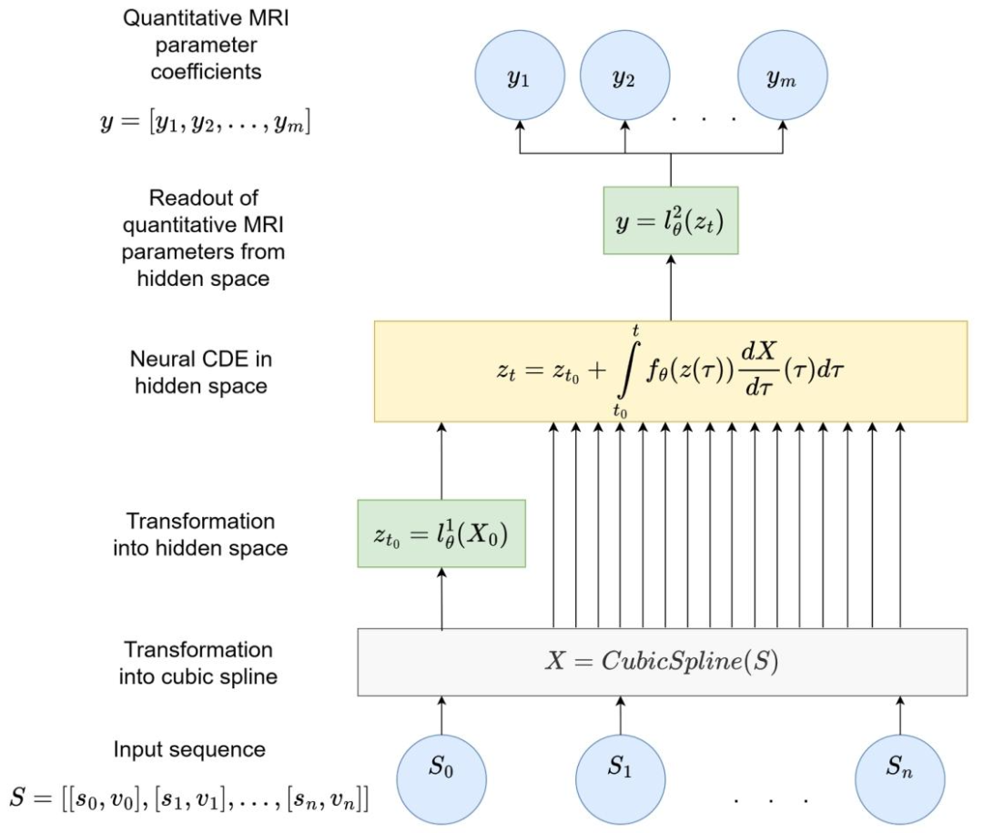
Fig. 1. Schematic representation of an NCDE for QMRI parameter estimation. The NCDE is composed of three neural networks: l 1 ∅, f∅, and l 2 ∅. The input sequence S can have arbitrary length and irregular sampling intervals. The length of output vector ycorresponds to the number of predicted QMRI parameter coefficients. X is a twice continuously differentiable cubic spline, whose knots are the elements of S. z denotes the hidden state.、
图1 用于QMRI参数估计的神经控制微分方程(NCDE)示意图 该NCDE由三个神经网络构成,分别为l₁∅、f∅ 和l₂∅。输入序列S可具有任意长度,且采样间隔可不规则;输出向量y的长度与待预测的QMRI参数系数数量一致。X代表二次连续可微的三次样条曲线,其节点为输入序列S的元素;z表示隐藏状态。
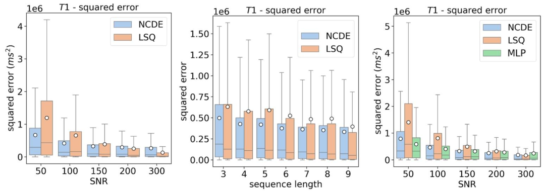
Fig. 2. Left: box plots of squared errors of estimated T1 parameters as a function of SNR for NCDE (blue) and LSQ (orange). Center: box plots of squared errors of estimated T1 parameters as a function of sequence length for NCDE (blue) and LSQ (orange). Acquisition-specific MLPs cannot be evaluated at variable acquisition schemes (left and center image). Right: box plots of squared errors of estimated T1 parameters as a function of SNR for NCDE (blue), LSQ (orange) and MLP (green), evaluated at a fixed acquisition scheme (1, 6, 10, 25◦). The white circle represents the mean squared error.
图2 可变翻转角T1映射(VFA T1-mapping)的T1估计误差平方箱线图 - 左图:以信噪比(SNR)为变量,展示神经控制微分方程(NCDE,蓝色)与最小二乘拟合(LSQ,橙色)的T1估计误差平方箱线图。 - 中图:以序列长度为变量,展示NCDE(蓝色)与LSQ(橙色)的T1估计误差平方箱线图。需注意,特定于采集协议的多层感知器(MLPs)无法在可变采集方案下评估(故左图与中图未纳入MLPs结果)。 - 右图:在固定采集方案(翻转角为1°, 6°, 10°, 25°)下,以SNR为变量,展示NCDE(蓝色)、LSQ(橙色)与MLP(绿色)的T1估计误差平方箱线图。图中白色圆点代表均方误差。
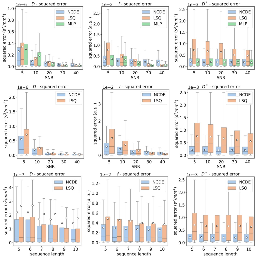
Fig. 3. Top row: box plots of squared errors of estimated IVIM parameters as a function of SNR for NCDE (blue), LSQ (orange) and MLP (green), evaluated at a fixed acquisition scheme (0, 10, 20, 50, 100, 300, 600 s/mm2). Middle row: box plots of squared errors of estimated IVIM parameters as a function of SNR for NCDE (blue) and LSQ (orange). Bottom row: box plots of squared errors of estimated IVIM parameters as a function of sequence length for NCDE (blue) and LSQ (orange). Acquisition-specific MLPs cannot be evaluated at variable acquisition schemes (middle and bottom rows). The white circle represents the mean squared error
图3 体素内不相干运动(IVIM)参数估计误差平方箱线图 - 上行图:在固定采集方案(b值为0, 10, 20, 50, 100, 300, 600 s/mm²)下,以信噪比(SNR)为变量,展示神经控制微分方程(NCDE,蓝色)、最小二乘拟合(LSQ,橙色)与多层感知器(MLP,绿色)的IVIM参数估计误差平方箱线图。 - 中行图:以SNR为变量,展示NCDE(蓝色)与LSQ(橙色)的IVIM参数估计误差平方箱线图。 - 下行图:以序列长度为变量,展示NCDE(蓝色)与LSQ(橙色)的IVIM参数估计误差平方箱线图。需注意,特定于采集协议的MLP无法在可变采集方案下评估(故中行图与下行图未纳入MLP结果)。 图中白色圆点代表均方误差。
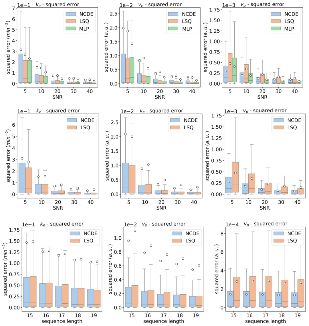
Fig. 4. Top row: box plots of squared errors of estimated DCE parameters as a function of SNR for NCDE (blue), LSQ (orange) and MLP (green), evaluated at a fixed acquisition scheme (9, 18, 27, 36, 45, 54, 63, 72, 81, 90, 99, 108, 117, 126, 135, 144, 153 s). Middle row: box plots of squared errors of estimated DCE parameters as a function of SNR for NCDE (blue) and LSQ (orange). Bottom row: box plots of squared errors of estimated DCE parameters as a function of sequence length for NCDE (blue) and LSQ (orange). Acquisition-specific MLPs cannot be evaluated at variable acquisition schemes (middle and bottom rows). The white circle represents the mean squared error
图4 动态对比增强(DCE)MRI参数估计误差平方箱线图 - 上行图:在固定采集方案(时间点为9, 18, 27, 36, 45, 54, 63, 72, 81, 90, 99, 108, 117, 126, 135, 144, 153秒)下,以信噪比(SNR)为变量,展示神经控制微分方程(NCDE,蓝色)、最小二乘拟合(LSQ,橙色)与多层感知器(MLP,绿色)的DCE参数估计误差平方箱线图。 - 中行图:以SNR为变量,展示NCDE(蓝色)与LSQ(橙色)的DCE参数估计误差平方箱线图。 - 下行图:以序列长度为变量,展示NCDE(蓝色)与LSQ(橙色)的DCE参数估计误差平方箱线图。需注意,特定于采集协议的MLP无法在可变采集方案下评估(故中行图与下行图未纳入MLP结果)。 图中白色圆点代表均方误差。
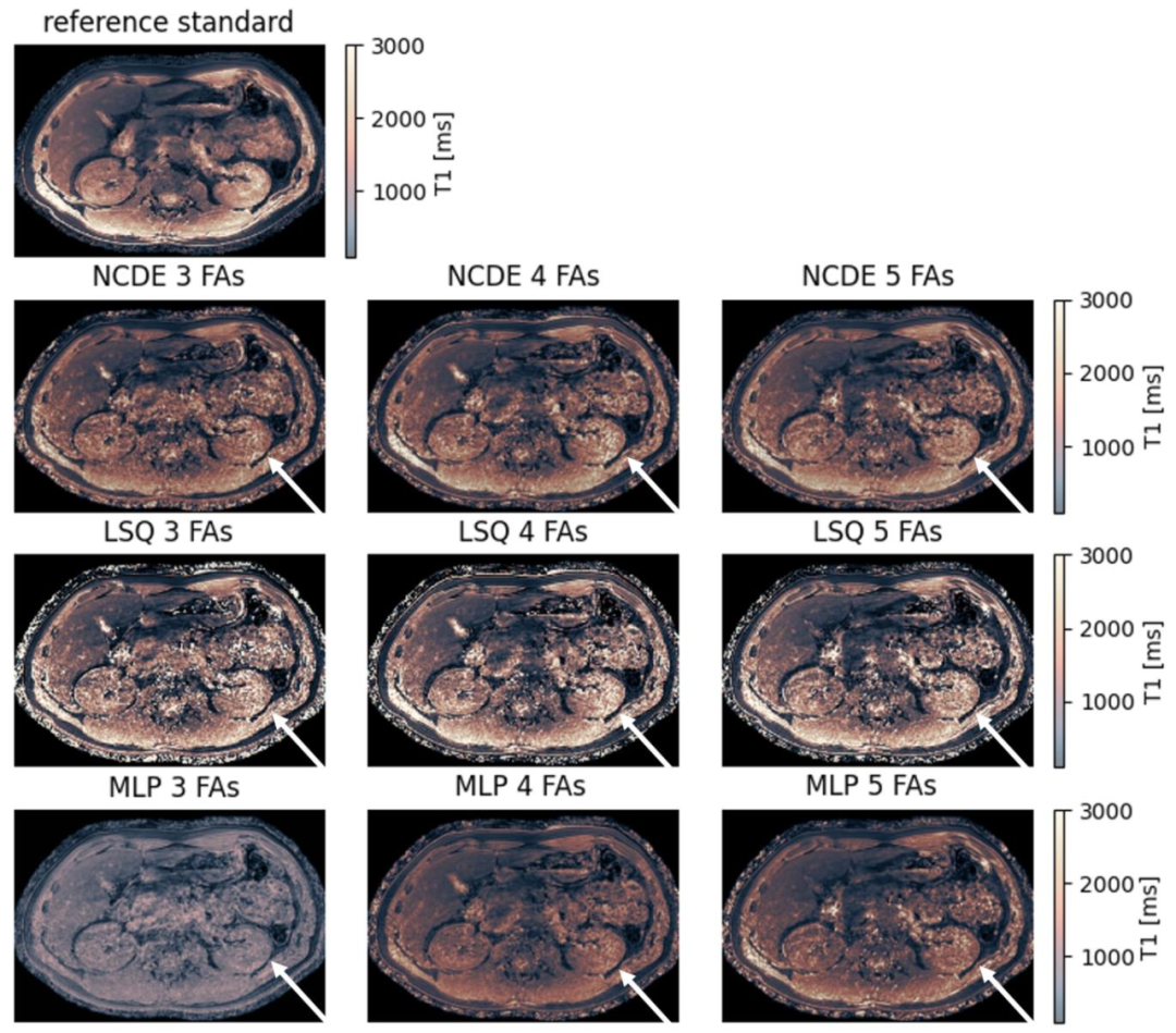
Fig. 5. Comparison of NCDE-based, LSQ-based and MLP-based abdominal T1 parameter maps based on subsampled data: abdomen reference T1 parameter map (top row) and estimated T1 parameter maps for NCDE (2nd row from the top), LSQ (3rd row from the top) and MLP (bottom row). Arrows indicate a region (left kidney) where T1 parameter maps were degraded by noise, affecting LSQ fitting parameter maps more than NCDE-based parameter maps. MLP-based T1 parameter maps suffer from poor contrast at 3 and 4 flip angles. Flip angles used for the evaluation at 3, 4 and 5 flip angles were 1, 6, 29◦, 1, 6, 15, 29◦ and 1, 6, 10, 20, 29◦, respectively
图5 基于子采样数据的腹部T1参数图对比:NCDE、LSQ与MLP方法 - 顶行:腹部T1参数参考图(作为真实值对照)。 - 第二行:基于神经控制微分方程(NCDE)估计的腹部T1参数图。 - 第三行:基于最小二乘拟合(LSQ)估计的腹部T1参数图。 - 底行:基于多层感知器(MLP)估计的腹部T1参数图。 图中箭头标注区域(左肾)为受噪声影响导致T1参数图质量下降的区域,其中LSQ拟合的参数图受噪声影响程度显著大于NCDE方法的参数图。此外,在使用3个和4个翻转角的评估场景中,MLP方法生成的T1参数图存在对比度不佳的问题。 本实验中,3个、4个及5个翻转角评估场景所使用的具体翻转角分别为1°, 6°, 29°、1°, 6°, 15°, 29°和1°, 6°, 10°, 20°, 29°。
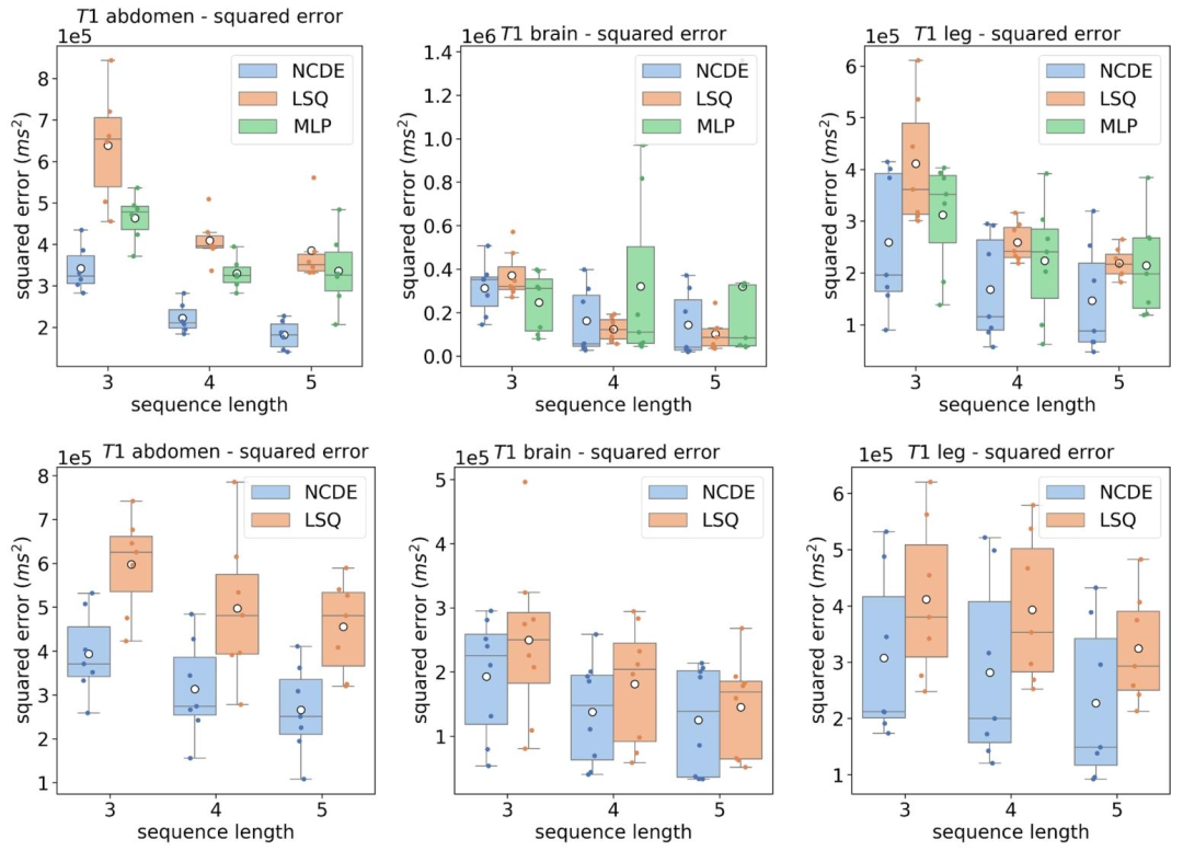
Fig. 6. Top row: box plot of mean squared errors per volunteer of the estimated T1 parameter by NCDEs (blue), LSQ (orange) and MLP (green) as a function of sequence length, grouped per anatomical region. Flip angles used for the evaluation at 3, 4 and 5 flip angles were 1, 6, 29◦, 1, 6, 15, 29◦ and 1, 6, 10, 20, 29◦, respectively. Bottom row: box plot of mean squared errors per volunteer of the estimated T1 parameter by NCDEs (blue), LSQ (orange) as a function of sequence length, grouped per anatomical region. Acquisition-specific MLPs cannot be evaluated at variable acquisition schemes (bottom row). The white circle represents the mean squared error over all volunteers
图6 不同解剖区域、不同序列长度下T1参数估计的志愿者人均均方误差箱线图 - 上行图:按解剖区域分组,以序列长度为变量,展示神经控制微分方程(NCDE,蓝色)、最小二乘拟合(LSQ,橙色)与多层感知器(MLP,绿色)估计T1参数的志愿者人均均方误差箱线图。其中,3个、4个及5个翻转角评估场景所用的翻转角分别为1°, 6°, 29°、1°, 6°, 15°, 29°和1°, 6°, 10°, 20°, 29°。 - 下行图:按解剖区域分组,以序列长度为变量,展示NCDE(蓝色)与LSQ(橙色)估计T1参数的志愿者人均均方误差箱线图。需注意,特定于采集协议的MLP无法在可变采集方案下评估(故下行图未纳入MLP结果)。 图中白色圆点代表所有志愿者的平均均方误差。
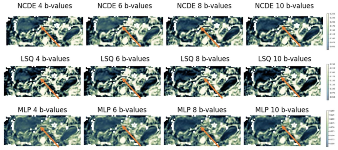
Fig. 7. Comparison of NCDE-based, LSQ-based and MLP-based abdominal perfusion fraction (f) parameter maps based on subsampled data: estimated f parameter maps for NCDE (top row), LSQ (middle row) and MLP (bottom row). Arrows indicate a region (liver) where perfusion fraction parameter maps were inconsistent between different subsets of b-values, affecting LSQ fitting parameter maps more than NCDE-based and MLP-based parameter maps. B-values used for the evaluation at 4, 6, 8 and 10 b-values were 0, 10, 50, 600 s/mm2, 0, 10, 20, 50, 75, 600 s/mm2, 0, 10, 20, 50, 75, 150, 400, 600 s/mm2 and 0, 10, 20, 30, 50, 75, 150, 250, 400, 600 s/mm2, respectively
图7 基于子采样数据的腹部灌注分数(f)参数图对比:NCDE、LSQ与MLP方法 - 顶行:基于神经控制微分方程(NCDE)估计的腹部灌注分数(f)参数图。 - 中行:基于最小二乘拟合(LSQ)估计的腹部灌注分数(f)参数图。 - 底行:基于多层感知器(MLP)估计的腹部灌注分数(f)参数图。 图中箭头标注区域(肝脏)为不同b值子集间灌注分数参数图存在一致性差异的区域,其中LSQ拟合的参数图受该差异影响程度显著大于NCDE和MLP方法的参数图。 本实验中,4个、6个、8个及10个b值评估场景所使用的具体b值分别为0, 10, 50, 600 s/mm²、0, 10, 20, 50, 75, 600 s/mm²、0, 10, 20, 50, 75, 150, 400, 600 s/mm²和0, 10, 20, 30, 50, 75, 150, 250, 400, 600 s/mm²。
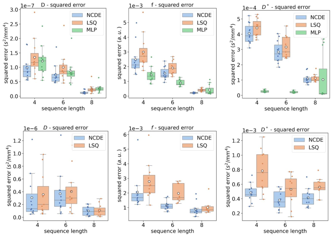
Fig. 8. Top row: box plot of mean squared errors per volunteer of the estimated IVIM parameters by NCDEs (blue), LSQ (orange) and MLP (green) as a function of sequence length. B-values used for the evaluation at 4, 6, 8 and 10 b-values were 0, 10, 50, 600 s/mm2, 0, 10, 20, 50, 75, 600 s/mm2, 0, 10, 20, 50, 75, 150, 400, 600 s/mm2 and 0, 10, 20, 30, 50, 75, 150, 250, 400, 600 s/mm2, respectively. Bottom row: box plot of mean squared errors per volunteer of the estimated IVIM parameter by NCDEs (blue), LSQ (orange) as a function of sequence length. Acquisition-specific MLPs cannot be evaluated at variable acquisition schemes. The white circle represents the mean squared error over all volunteers.
图8 不同序列长度下IVIM参数估计的志愿者人均均方误差箱线图 - 上行图:以序列长度为变量,展示神经控制微分方程(NCDE,蓝色)、最小二乘拟合(LSQ,橙色)与多层感知器(MLP,绿色)估计IVIM参数的志愿者人均均方误差箱线图。其中,4个、6个、8个及10个b值评估场景所用的b值分别为0, 10, 50, 600 s/mm²、0, 10, 20, 50, 75, 600 s/mm²、0, 10, 20, 50, 75, 150, 400, 600 s/mm²和0, 10, 20, 30, 50, 75, 150, 250, 400, 600 s/mm²。 - 下行图:以序列长度为变量,展示NCDE(蓝色)与LSQ(橙色)估计IVIM参数的志愿者人均均方误差箱线图。需注意,特定于采集协议的MLP无法在可变采集方案下评估(故下行图未纳入MLP结果)。 图中白色圆点代表所有志愿者的平均均方误差。
Table
表
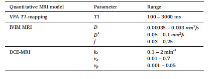
Table 1 Description of QMRI parameter ranges used in simulated data during training and evaluation. QMRI parameters were randomly sampled from a uniform distribution with these ranges.
表1 训练与评估阶段模拟数据中所用QMRI参数的取值范围说明 QMRI参数均从符合以下取值范围的均匀分布中随机采样得到。
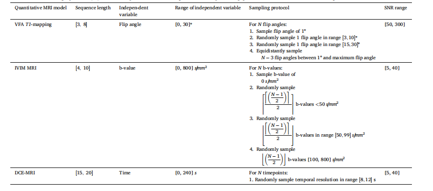
Table 2 Description of the protocol for sampling the independent variables and simulating the corresponding signal curves. These simulation procedures have been used during training and evaluation. Even though the denoted range in SNR appears vastly different among the three QMRI simulations, this is caused by differences in the SNR definition. The ceiling operator (⌈x⌉) rounds x up to the nearest integer, the floor operator (⌊x⌋) rounds x down to the nearest integer.
表2 自变量采样及对应信号曲线模拟的协议说明 上述模拟流程均用于训练与评估阶段。尽管三种QMRI模拟中所示的信噪比(SNR)范围看似差异显著,但这是由信噪比定义的不同所致。上取整运算符(⌈x⌉)将x向上取整至最接近的整数,下取整运算符(⌊x⌋)将x向下取整至最接近的整数。
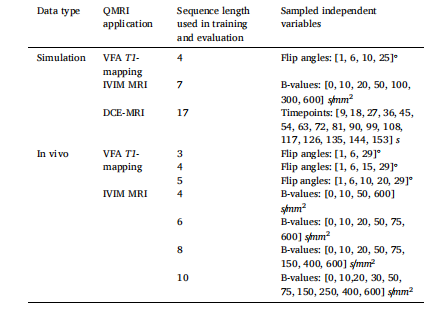
Table 3Description of the sampled independent variables for training of the MLPs and for the fixed-acquisition evaluations of the MLPs, NCDEs and LSQ fitting.
表3 多层感知器(MLPs)训练所用的自变量采样说明,以及多层感知器(MLPs)、神经控制微分方程(NCDEs)和最小二乘拟合(LSQ fitting)在固定采集协议评估中的自变量采样说明