计算机视觉让机器具备了"看懂"世界的能力,能从图像的像素点中提炼出物体的轮廓与语义。
而自然语言处理中的序列模型,则赋予机器"听懂"与"理解"人类语言的本领。
两者的区别在于,前者侧重于空间结构的处理,后者则聚焦于时间序列的解读。
接下来,我们将深入探讨序列模型如何逐步揭示语言背后的深层规律。
1. 序列模型
什么是序列模型?
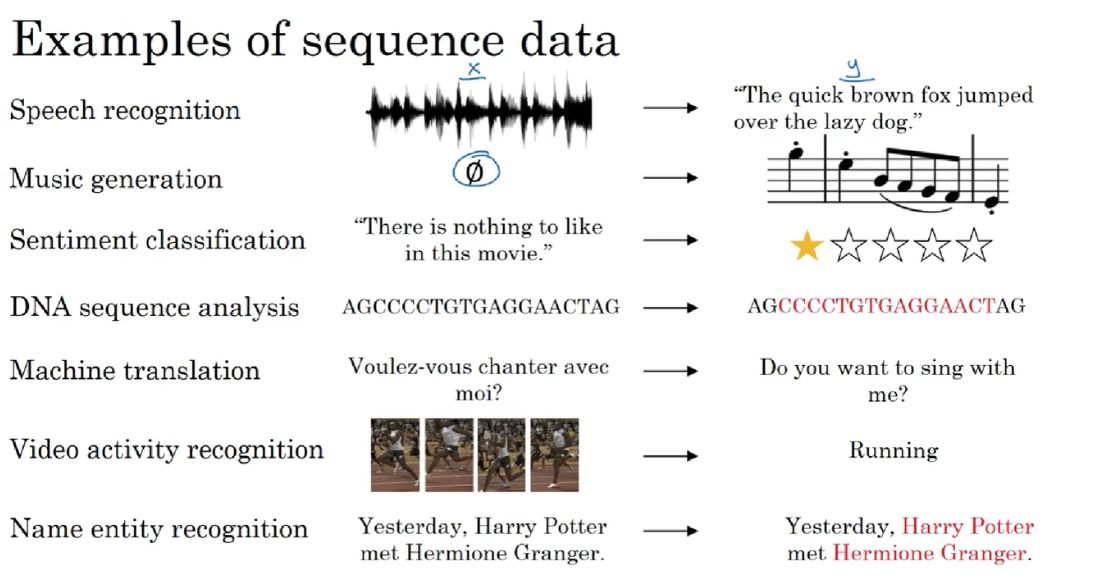
序列模型是一类专门处理动态、有序序列数据的工具,它能捕捉序列中元素间的关系,如因果、对齐等,进而进行预测、生成或分类。在自然语言处理、语音识别等领域,序列模型被广泛应用,像文本生成、机器翻译、语音识别等任务都依赖它来处理语言的动态模式。
早期的循环神经网络RNN是序列模型的代表,但如今Transformer等更先进的模型在更大的数据集上已逐渐取代RNN,成为主流。
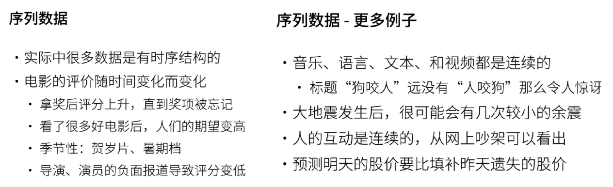
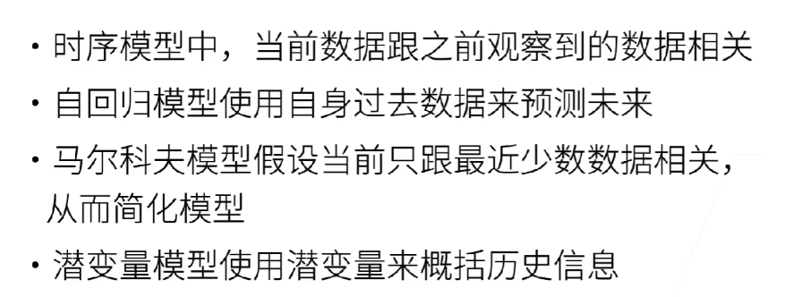
处理序列数据(如时间序列、语言)的关键是利用历史信息预测未来。
以下是两种主流的建模思想:
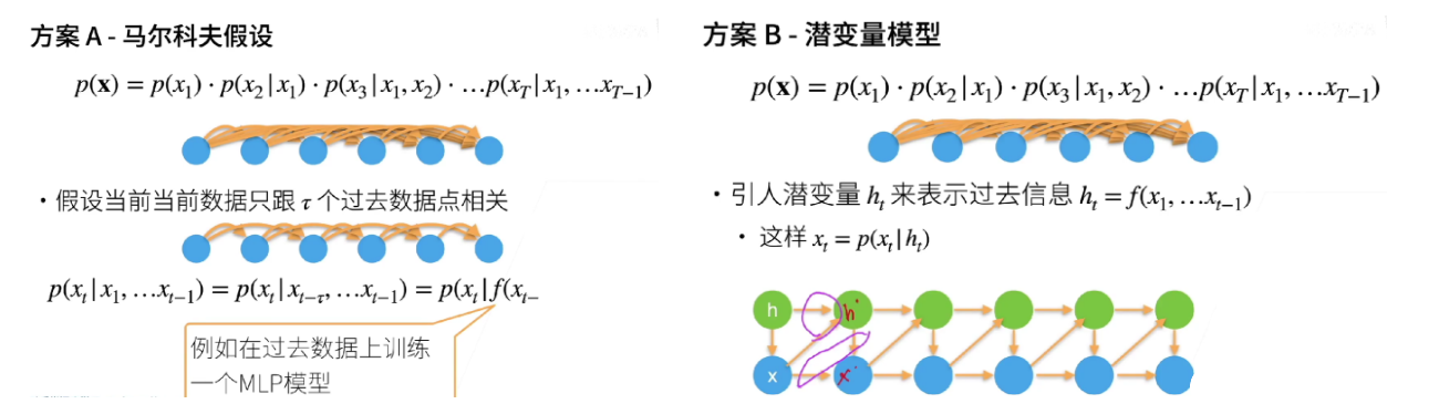
1.1 马尔科夫假设:有限的短期记忆
核心思想 :假设"未来只与最近的过去有关",强行忽略更早的历史。这是一个简化历史的策略。
-
怎么做 :模型只使用最近
n个数据点来预测下一个点。例如,n-gram语言模型或时间序列中的AR(n)模型。 -
优点 :简单、高效、易解释。
-
缺点 :无法捕捉长期依赖 关系,且选择合适的记忆长度
n很困难。 -
好比 :一条记忆力只有几秒的金鱼,只记得刚才发生的事。
1.2 潜变量模型:无限的摘要记忆
核心思想 :引入一个内部的隐状态(潜变量) 来动态地概括整个历史 。这是一个摘要历史的策略。
-
怎么做:模型拥有一个"记忆单元"(潜变量),它随着新数据的到来而不断更新。预测完全基于这个包含了所有历史精华的记忆单元。递归神经网络(RNN、LSTM)、隐马尔可夫模型(HMM)都属于此类。
-
优点 :理论上能捕捉无限长期的依赖,模型能力更强。
-
缺点 :模型复杂、难以训练、可解释性差。
-
好比 :一位有秘书的CEO。CEO(模型)不记细节,但秘书(潜变量)会为他维护一份持续更新的摘要备忘录,所有决策都基于这份高效的备忘录。
总结:
1.3 代码实例
首先,我们生成一些数据。
使用正弦函数和一些可加性噪声来生成序列数据,时间步为:1,2,......,1000:
%matplotlib inline
import torch
from torch import nn
from d2l import torch as d2l

T = 1000  # 总共产生1000个点
time = torch.arange(1, T + 1, dtype=torch.float32)
x = torch.sin(0.01 * time) + torch.normal(0, 0.2, (T,))
d2l.plot(time, [x], 'time', 'x', xlim=[1, 1000], figsize=(6, 3))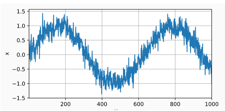
接下来,我们将这个序列转换为模型的特征-标签(feature-label)对。
数据对是: y_t = x_t 和 \mathbf{x}_t = x_{t-\\tau}, \\ldots, x_{t-1}。
使用的是方案1的马尔科夫假设,在这里,我们仅使用前600个"特征-标签"对进行训练。:
tau = 4
features = torch.zeros((T - tau, tau))
for i in range(tau):
    features[:, i] = x[i: T - tau + i]
labels = x[tau:].reshape((-1, 1))

batch_size, n_train = 16, 600
# 只有前n_train个样本用于训练
train_iter = d2l.load_array((features[:n_train], labels[:n_train]),
                            batch_size, is_train=True)

features的值大致为:
[[1, 2, 3, 4],
 [2, 3, 4, 5],
 [3, 4, 5, 6],
 [4, 5, 6, 7]]

 labels的值大致为:
 [[5],
 [6],
 [7],
 [8]]
在这里,我们使用一个相当简单的架构训练模型。
一个拥有两个全连接层的多层感知机,ReLU激活函数和平方损失。
# 初始化网络权重的函数
def init_weights(m):
    if type(m) == nn.Linear:
        nn.init.xavier_uniform_(m.weight)

# 一个简单的多层感知机
def get_net():
    net = nn.Sequential(nn.Linear(4, 10),
                        nn.ReLU(),
                        nn.Linear(10, 1))
    net.apply(init_weights)
    return net

# 平方损失。注意:MSELoss计算平方误差时不带系数1/2
loss = nn.MSELoss(reduction='none')
训练代码:
def train(net, train_iter, loss, epochs, lr):
trainer = torch.optim.Adam(net.parameters(), lr)
for epoch in range(epochs):
for X, y in train_iter:
trainer.zero_grad()
l = loss(net(X), y)
l.sum().backward()
trainer.step()
print(f'epoch {epoch + 1}, '
f'loss: {d2l.evaluate_loss(net, train_iter, loss):f}')
net = get_net()
train(net, train_iter, loss, 5, 0.01)
输出:
epoch 1, loss: 0.076846
epoch 2, loss: 0.056340
epoch 3, loss: 0.053779
epoch 4, loss: 0.056320
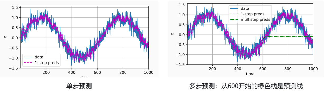
epoch 5, loss: 0.051650首先检查模型预测下一个时间步的能力, 也就是单步预测(one-step-ahead prediction)。
onestep_preds = net(features)
d2l.plot([time, time[tau:]],
         [x.detach().numpy(), onestep_preds.detach().numpy()], 'time',
         'x', legend=['data', '1-step preds'], xlim=[1, 1000],
         figsize=(6, 3))
使用我们自己的预测(而不是原始数据)来进行多步预测:
multistep_preds = torch.zeros(T)
multistep_preds[: n_train + tau] = x[: n_train + tau]
for i in range(n_train + tau, T):
    multistep_preds[i] = net(
        multistep_preds[i - tau:i].reshape((1, -1)))

d2l.plot([time, time[tau:], time[n_train + tau:]],
         [x.detach().numpy(), onestep_preds.detach().numpy(),
          multistep_preds[n_train + tau:].detach().numpy()], 'time',
         'x', legend=['data', '1-step preds', 'multistep preds'],
xlim=[1, 1000], figsize=(6, 3))-
单步预测 :在单步预测的情况下,模型是基于真实的历史数据来预测下一个时间步的值。例如,输入
[1, 2, 3, 4]预测下一个值,输入[2, 3, 4, 5]预测再下一个值,以此类推。每个预测都是独立进行的,基于真实的历史数据。 -
多步预测:在多步预测中,模型需要递归地使用之前预测的结果作为后续预测的输入。例如:
-
初始输入
[1, 2, 3, 4],预测出6。 -
下一次输入则是
[2, 3, 4, 6],基于这个输入预测下一个值是9。 -
然后输入变为
[3, 4, 6, 9],继续预测。
-
通过对整个序列预测的计算, 让我们更仔细地看一下k步预测的困难。
max_steps = 64

features = torch.zeros((T - tau - max_steps + 1, tau + max_steps))
# 列i(i<tau)是来自x的观测,其时间步从(i)到(i+T-tau-max_steps+1)
for i in range(tau):
    features[:, i] = x[i: i + T - tau - max_steps + 1]

# 列i(i>=tau)是来自(i-tau+1)步的预测,其时间步从(i)到(i+T-tau-max_steps+1)
for i in range(tau, tau + max_steps):
    features[:, i] = net(features[:, i - tau:i]).reshape(-1)

steps = (1, 4, 16, 64)
d2l.plot([time[tau + i - 1: T - max_steps + i] for i in steps],
         [features[:, (tau + i - 1)].detach().numpy() for i in steps], 'time', 'x',
         legend=[f'{i}-step preds' for i in steps], xlim=[5, 1000],
         figsize=(6, 3))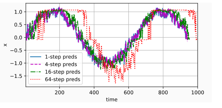
2. 文本预处理
2.1 文本清洗
这是最基础的步骤,旨在去除文本中的无关字符和格式。
-
操作:
-
移除HTML/XML标签、超链接、特殊字符(如
#,@,<)。 -
处理或删除数字(如将数字统一替换为
<NUM>标签,或直接删除)。 -
纠正明显的拼写错误(可选,需要额外工具)。
-
统一大小写(通常转为小写,以消除"Apple"和"apple"的区别)。
-
2.2 分词
将连续的文本序列切分成有意义的单元(通常是单词或子词)的过程。
-
操作:
-
对于英文等以空格分隔的语言,使用空格和标点符号进行分割相对简单。例如,
"I love NLP!"->["I", "love", "NLP", "!"]。 -
对于中文、日文等没有空格分隔的语言,分词是一个复杂问题,需要专门的分词工具(如Jieba for Chinese)。例如,
"我爱自然语言处理"->["我", "爱", "自然语言处理"]。
-
2.3 文本标准化
将单词的不同形态统一为其基本形式,以减少词汇冗余。
-
操作:
-
词干提取 :一种粗糙的启发式方法,直接砍掉词缀以获得词干。速度快但不精确。例如,
"running"->"run","flies"->"fli"。 -
词形还原 :基于词典和语法分析,将单词还原为字典中的标准形式( lemma)。更准确但计算成本更高。例如,
"running"->"run","was"->"be","better"->"good"。 -
注 :在大多数应用中,词形还原是比词干提取更好的选择。
-
2.4 文本过滤
移除对任务目标贡献不大的词汇,进一步精简数据。
-
操作:
-
去除停用词 :删除在语言中非常常见但含义空洞的词(如 "the", "a", "an", "in", "of")。这对于信息检索、主题建模等任务非常有效。但对于情感分析或机器翻译等任务,停用词可能很重要,需要谨慎处理。
-
去除低频/高频词:移除在整个语料库中出现次数极少(可能为拼写错误)或极多(可能为通用词)的词汇。
-
2.5 文本向量化/表示学习(数值化)
这是最后一步,也是至关重要的一步,将处理好的文本令牌转换为模型可读的数值向量。
-
常见方法:
-
词袋模型:将文本表示为一个长向量,向量的每个维度代表一个词,值代表该词是否出现或出现的次数。它忽略了词的顺序。
-
TF-IDF:对词袋模型的改进,不仅考虑词频,还考虑词的"重要性"(逆文档频率),以降低常见词的权重。
-
词嵌入:如Word2Vec、GloVe、FastText。它将单词映射到低维稠密向量空间中,语义相似的词在向量空间中的位置也更接近。这是现代深度学习模型的主流方法。
-
上下文嵌入:如BERT、ELMo等模型生成的向量,能够根据上下文为同一个词生成不同的向量表示,效果最佳。
-
2.6 代码实例
本节中,我们将解析文本的常见预处理步骤。 这些步骤包括:
-
将文本作为字符串加载到内存中。
-
将字符串拆分为词元(如单词和字符)。
-
建立一个词表,将拆分的词元映射到数字索引。
-
将文本转换为数字索引序列,方便模型操作。
import collections
import re
from d2l import torch as d2l
读取数据集:
#@save
d2l.DATA_HUB['time_machine'] = (d2l.DATA_URL + 'timemachine.txt',
                                '090b5e7e70c295757f55df93cb0a180b9691891a')

def read_time_machine():  #@save
    """将时间机器数据集加载到文本行的列表中"""
    with open(d2l.download('time_machine'), 'r') as f:
        lines = f.readlines()
    return [re.sub('[^A-Za-z]+', ' ', line).strip().lower() for line in lines]

lines = read_time_machine()
print(f'文本总行数: {len(lines)}')
print(lines[0])
print(lines[10])

输出:
Downloading ../data/timemachine.txt from http://d2l-data.s3-accelerate.amazonaws.com/timemachine.txt ...
文本总行数: 3221
the time machine by h g wells
twinkled and his usually pale face was flushed and animated the
词元化:
tokenize函数将文本行列表(lines)作为输入, 列表中的每个元素是一个文本序列(如一条文本行)。
每个文本序列又被拆分成一个词元列表,词元(token)是文本的基本单位。 最后,返回一个由词元列表组成的列表,其中的每个词元都是一个字符串(string)。
def tokenize(lines, token='word'):  #@save
    """将文本行拆分为单词或字符词元"""
    if token == 'word':
        return [line.split() for line in lines]
    elif token == 'char':
        return [list(line) for line in lines]
    else:
        print('错误:未知词元类型:' + token)

tokens = tokenize(lines)
for i in range(11):
    print(tokens[i])

输出:
['the', 'time', 'machine', 'by', 'h', 'g', 'wells']
[]
[]
[]
[]
['i']
[]
[]
['the','time','traveller','for','so','it','will','be','convenient','to','speak','of','him']
['was','expounding','a','recondite','matter','to','us','his','grey','eyes','shone','and']
['twinkled','and','his','usually','pale','face','was','flushed','and','animated','the']
词表:
词元的类型是字符串,而模型需要的输入是数字,因此这种类型不方便模型使用。
现在,让我们构建一个字典,通常也叫做词表(vocabulary), 用来将字符串类型的词元映射到从0开始的数字索引中。
class Vocab:  #@save
    """文本词表"""
    def __init__(self, tokens=None, min_freq=0, reserved_tokens=None):
        if tokens is None:
            tokens = []
        if reserved_tokens is None:
            reserved_tokens = []
        # 按出现频率排序
        counter = count_corpus(tokens)
        self._token_freqs = sorted(counter.items(), key=lambda x: x[1],reverse=True)
        # 未知词元的索引为0
        self.idx_to_token = ['<unk>'] + reserved_tokens
        self.token_to_idx = {token: idx
                             for idx, token in enumerate(self.idx_to_token)}
        for token, freq in self._token_freqs:
            if freq < min_freq:
                break
            if token not in self.token_to_idx:
                self.idx_to_token.append(token)
                self.token_to_idx[token] = len(self.idx_to_token) - 1

    def __len__(self):
        return len(self.idx_to_token)

    def __getitem__(self, tokens):
        if not isinstance(tokens, (list, tuple)):
            return self.token_to_idx.get(tokens, self.unk)
        return [self.__getitem__(token) for token in tokens]

    def to_tokens(self, indices):
        if not isinstance(indices, (list, tuple)):
            return self.idx_to_token[indices]
        return [self.idx_to_token[index] for index in indices]

    @property
    def unk(self):  # 未知词元的索引为0
        return 0

    @property
    def token_freqs(self):
        return self._token_freqs

def count_corpus(tokens):  #@save
    """统计词元的频率"""
    # 这里的tokens是1D列表或2D列表
    if len(tokens) == 0 or isinstance(tokens[0], list):
        # 将词元列表展平成一个列表
        tokens = [token for line in tokens for token in line]
    return collections.Counter(tokens)
使用
enumerate可以避免手动维护一个计数器来记录索引,使代码更加简洁易读。list = 'a', 'b', 'c', 'd'
for index, value in enumerate(list):
print(index, value)
输出结果为:
0 a
1 b
2 c
3 d
我们首先使用时光机器数据集作为语料库来构建词表,然后打印前几个高频词元及其索引。
vocab = Vocab(tokens)
print(list(vocab.token_to_idx.items())[:10])

输出:
[('<unk>', 0), ('the', 1), ('i', 2), ('and', 3), ('of', 4), ('a', 5), ('to', 6), ('was', 7), ('in', 8), ('that', 9)]
将每一条文本行转换成一个数字索引列表。
for i in [0, 10]:
    print('文本:', tokens[i])
    print('索引:', vocab[tokens[i]])

输出:
文本: ['the', 'time', 'machine', 'by', 'h', 'g', 'wells']
索引: [1, 19, 50, 40, 2183, 2184, 400]
文本: ['twinkled', 'and', 'his', 'usually', 'pale', 'face', 'was', 'flushed', 'and', 'animated', 'the']
索引: [2186, 3, 25, 1044, 362, 113, 7, 1421, 3, 1045, 1]
整合所有功能:
在使用上述函数时,我们将所有功能打包到load_corpus_time_machine函数中, 该函数返回corpus(词元索引列表)和vocab(时光机器语料库的词表)。 我们在这里所做的改变是:
-
为了简化后面章节中的训练,我们使用字符(而不是单词)实现文本词元化;
-
时光机器数据集中的每个文本行不一定是一个句子或一个段落,还可能是一个单词,因此返回的
corpus仅处理为单个列表,而不是使用多词元列表构成的一个列表。def load_corpus_time_machine(max_tokens=-1): #@save
"""返回时光机器数据集的词元索引列表和词表"""
lines = read_time_machine()
tokens = tokenize(lines, 'char')
vocab = Vocab(tokens)
# 因为时光机器数据集中的每个文本行不一定是一个句子或一个段落,
# 所以将所有文本行展平到一个列表中
corpus = [vocab[token] for line in tokens for token in line]
if max_tokens > 0:
corpus = corpus[:max_tokens]
return corpus, vocabcorpus, vocab = load_corpus_time_machine()
len(corpus), len(vocab)输出:(170580, 28)