Deep Learning|01 RBF Network

Deep Learning|01 RBF Network

文章目录

• [Deep Learning|01 RBF Network](#Deep Learning|01 RBF Network)
• • [Radial Basis Function Interpolation, RBF Interpolation](#Radial Basis Function Interpolation, RBF Interpolation)
  • [RBF Network](#RBF Network)
  • [How to build a simple RBF network?](#How to build a simple RBF network?)

Radial Basis Function Interpolation, RBF Interpolation

Radial basis functions are a class of real-valued functions that depend solely on the radial distance between the input vector and a fixed center point. Their core characteristic is that the function value is independent of the direction of the input and only related to the distance from the input to the center point.

Let Φ ( x ) \Phi (x) Φ(x) is a RBF , for any input vector x \boldsymbol{x} x , and center vectors c \boldsymbol{c} c ,we define Φ ( x ) \Phi (x) Φ(x) uesd Gauss functon :

Φ ( x ) = e − β ∥ x − c ∥ 2 \Phi(\boldsymbol{x})=e^{-\beta \|\boldsymbol{x}-\boldsymbol{c}\|^2} Φ(x)=e−β∥x−c∥2

which β \beta β control the width of Gauss functon .

Note : It is not the only way. In fact, any similar δ \delta δ function is available.

Radial Basis Function Interpolation, RBF Interpolation , is essentially an interpolation method that use a linear combination of radial basis functions (RBFs) to

"exactly approximate" the function f ( x ) f(x) f(x) at known points.The formular is as follows:

f ( x ) = ∑ j = 1 n λ j Φ j ( x ) = ∑ j = 1 n λ j e − β j ∥ x − c j ∥ 2 f(x)= \sum_{j=1}^{n} \lambda_j\Phi_j (\boldsymbol{x})= \sum_{j=1}^{n} \lambda_je^{-\beta_j \|\boldsymbol{x}-\boldsymbol{c}_j\|^2} f(x)=j=1∑nλjΦj(x)=j=1∑nλje−βj∥x−cj∥2

This defination is like Maximum Likelihood Estimation 。This likely unrigorous？No! Brommehead and Lowe had given the proof of
RBF

. Magically!😊

RBF Network

Radial Basis Function Network (RBF Network) is a type of feedforward neural network with a single hidden layer. Its core feature is that it adopts "radial basis functions (RBFs)" as the activation functions of the hidden layer, and it is specifically used to solve supervised learning tasks such as nonlinear regression, pattern classification, and function approximation. Its key advantages lie in "strong local approximation capability, fast training speed, and stable generalization performance", making it widely applied in small and medium-sized nonlinear problems.

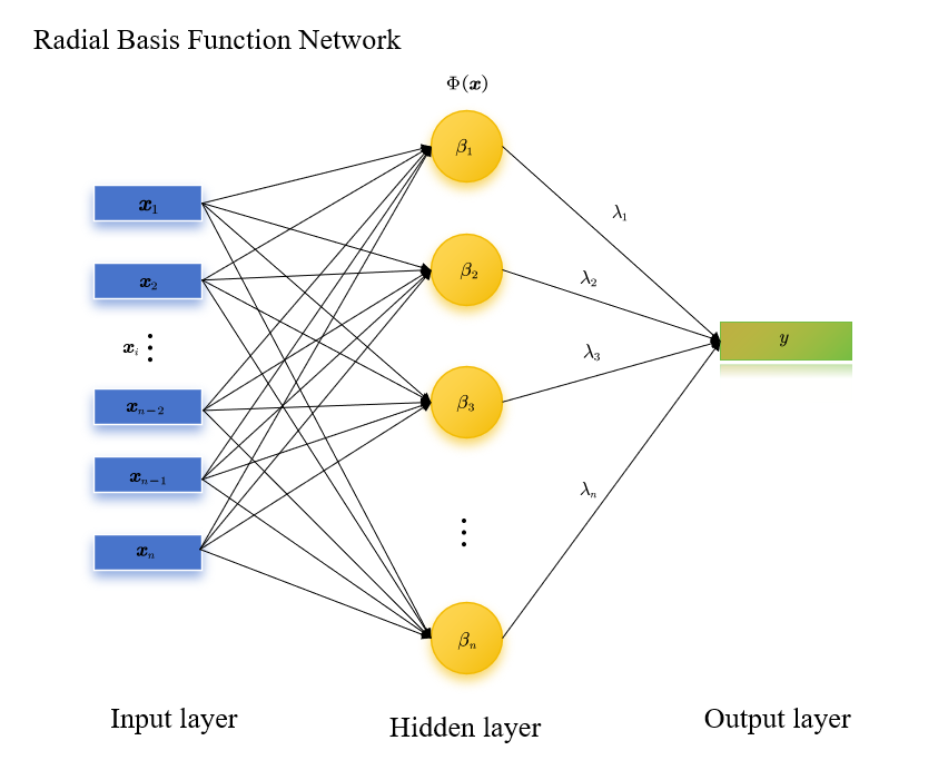
RBF Network = ∑ j = 1 n λ j Φ j ( x ) \text{RBF Network}=\sum_{j=1}^{n} \lambda_j\Phi_j (\boldsymbol{x}) RBF Network=j=1∑nλjΦj(x)

How to build a simple RBF network?

Aassuming we have series data { ( x , y ) } i = 1 n \{\left(\boldsymbol{x},y\right)\}{i=1}^n {(x,y)}i=1n , the training objective of an RBF network is to determine three types of parameters: hidden layer centers { c i } i n c \{\boldsymbol{c}i\}{i}^{n_c} {ci}inc, hidden layer widths { σ i } i n σ \{\sigma_i\}{i}^{n_\sigma} {σi}inσ, and output layer weights { w i } i n w \{w_i\}_{i}^{n_w} {wi}inw.

Step1: load data and K-means clustering

import pandas as pd
import numpy as np
import matplotlib.pyplot as plt
from sklearn.cluster import KMeans
from sklearn.preprocessing import StandardScaler
import os



def preprocess_data(data):

    data = data.dropna()
    if data.dtypes.iloc[-1] == 'object' or len(data.iloc[:, -1].unique()) < 10:
        X = data.iloc[:, :-1].values
        has_labels = True
        labels = data.iloc[:, -1].values
    else:
        X = data.values
        has_labels = False
        labels = None
    scaler = StandardScaler()
    X_scaled = scaler.fit_transform(X)
  
    return X_scaled, has_labels, labels
    
def perform_kmeans(X, n_clusters=neural_numbers, random_state=42):
    kmeans = KMeans(n_clusters=n_clusters, random_state=random_state)
    clusters = kmeans.fit_predict(X)
    centroids = kmeans.cluster_centers_
    return clusters, centroids

def visualize_results(X, original_labels, clusters, centroids, has_original_labels=False):

    fig, axes = plt.subplots(1, 2, figsize=(16, 8))
     has_original_labels and original_labels is not None:
        scatter1 = axes[0].scatter(X[:, 0], X[:, 1], c=original_labels, cmap='viridis', alpha=0.7)
        axes[0].set_title('oringal data distrbution', fontsize=14)
        plt.colorbar(scatter1, ax=axes[0], label='oringal lable')


scatter2 = axes[1].scatter(X[:, 0], X[:, 1], c=clusters, cmap='viridis', alpha=0.7)
    axes[1].scatter(centroids[:, 0], centroids[:, 1], s=300, c='red', marker='X', label='clustering center')
    axes[1].set_title('result of clustering', fontsize=14)
    plt.colorbar(scatter2, ax=axes[1], label='clustering label')
    axes[1].legend()
   for ax in axes:
        ax.set_xlabel('feature_1（标准化）', fontsize=12)
        ax.set_ylabel('feature_2（标准化）', fontsize=12)
        ax.grid(True, linestyle='--', alpha=0.6)
    
    plt.tight_layout()
 
    if not os.path.exists('results'):
        os.makedirs('results')
    plt.savefig('results/clustering_comparison.png', dpi=300, bbox_inches='tight')
    print("figures save to : results/clustering_comparison.png")
    
    plt.show()



def main(file_path, n_clusters=3):

    data = load_data(file_path)
    if data is None:
        return
    
    X, has_labels, original_labels = preprocess_data(data)
    

    if X.shape[1] > 2:
        from sklearn.decomposition import PCA
        print(f"data dimension is {X.shape[1]}，use PCA to 2-dimension to showase")
        pca = PCA(n_components=2)
        X = pca.fit_transform(X)
    

    clusters, centroids = perform_kmeans(X, n_clusters)
    

    visualize_results(X, original_labels, clusters, centroids, has_labels)

if __name__ == "__main__":




  datapath="data.csv"

  neural_numbers=3

  data = pd.read_csv(file_path) # Must .csv

  main(datapath, neural_numbers)

**Step2: Calculate the hidden layer widths **$

The widths do not require training and are usually calculated automatically based on the distribution of the centers.Most commonly used，adaptive calculation based on "nearest neighbor center distance"

For each center c j \boldsymbol{c}_j cj, first find another center c k \boldsymbol{c}_k ck that is closest to it ( k ≠ j k \neq j k=j), and denote this distance as d j d_j dj:

d j = min ⁡ k = 1 , 2 , . . . , n k ≠ j ∥ c j − c k ∥ d_j = \min_{\substack{k=1,2,...,n \\ k \neq j}} \|\boldsymbol{c}_j - \boldsymbol{c}_k\| dj=k=1,2,...,nk=jmin∥cj−ck∥

(where d j d_j dj represents the Euclidean distance from the j j j-th center to its nearest neighboring center)

Then, define β j \beta_j βj as a quantity related to d j d_j dj to ensure that the "effective range" of the RBF matches the distance between adjacent centers:

β j = 1 2 ⋅ d j 2 \beta_j = \frac{1}{2 \cdot d_j^2} βj=2⋅dj21

Step3: Solve for the output layer weights

After the centers { c i } \{\boldsymbol{c}_i\} {ci} and widths { σ i } \{\sigma_i\} {σi} are determined, the hidden layer output h i ( x ) h_i(\boldsymbol{x}) hi(x) can be regarded as a "fixed nonlinear feature". At this point, the solution for the output layer weights is transformed into a linear regression problem (gradient descent is not required, and the least squares method can be used directly).

Suppose the training set contains N N N samples ( x k , y k ) (\boldsymbol{x}_k, y_k) (xk,yk) (where y k y_k yk is the true label), and the network output is$ y ^ k = ∑ i = 1 m w i h i ( x k ) + w 0 \hat{y}k = \sum{i=1}^m w_i h_i(\boldsymbol{x}_k) + w_0 y^k=∑i=1mwihi(xk)+w0. By minimizing the "squared error between the predicted value and the true value":

L = ∑ k = 1 N ( y ^ k − y k ) 2 \mathcal{L} = \sum_{k=1}^N (\hat{y}_k - y_k)^2 L=k=1∑N(y^k−yk)2

This can be converted into the matrix equation H ⋅ w = y \mathbf{H} \cdot \boldsymbol{w} = \boldsymbol{y} H⋅w=y), where:

• H \mathbf{H} H is an N × ( m + 1 ) N \times (m+1) N×(m+1) "feature matrix", and each row is [ 1 , h 1 ( x k ) , h 2 ( x k ) , . . . , h m ( x k ) ] [1, h_1(\boldsymbol{x}_k), h_2(\boldsymbol{x}_k), ..., h_m(\boldsymbol{x}_k)] [1,h1(xk),h2(xk),...,hm(xk)] (the 1 corresponds to the bias term w 0 w_0 w0);
• w = [ w 0 , w 1 , . . . , w m ] T \boldsymbol{w} = [w_0, w_1, ..., w_m]^T w=[w0,w1,...,wm]T is the weight vector to be solved;
• y = [ y 1 , y 2 , . . . , y N ] T \boldsymbol{y} = [y_1, y_2, ..., y_N]^T y=[y1,y2,...,yN]T is the true label vector.

The weights are solved using the pseudoinverse matrix (to avoid the problem of matrix singularity):

w = ( H T H ) − 1 H T y \boldsymbol{w} = (\mathbf{H}^T \mathbf{H})^{-1} \mathbf{H}^T \boldsymbol{y} w=(HTH)−1HTy

This step is the key to the fast training of the RBF network --- linear problems can be solved directly without repeated iterations.
Later, we will construct a Radial Basis Function (RBF) network to accomplish the prediction task.