文章目录
摘要
本周继续上周的工作,学习ViT的论文,并通过代码测试可行性,Transformer在大数据的上限远比神经网络更高。
Abstract
This week, I continued the work from last week, studied the ViT paper, and tested its feasibility through code. Transformers have a much higher upper limit on big data compared to neural networks.
1 ViT
ViT是将transformer用于cv方向,transformer在nlp领域应用很好,Alexey等作者,将transfomer用于cv也得到不错的结果。论文是《An Image Is Worth 16x16 Words:Transformers For Image Recognition At Scale》
1.1 预处理
ViT要把图片分割成多个patch,然后将patch拉成向量,比如一个 224 × 224 t i m e s 3 224\times 224 times 3 224×224times3的图片,3代表通道,一个path的大小是 16 × 16 16\times 16 16×16,那么得到的就是196个 16 × 16 × 3 16 \times 16 \times 3 16×16×3大小的图像块。把这些图像块拉成向量,一个块有256个像素,然后三个通道,展平长度就是768,数据的形状就会变成(196,768)的大小,就解决了直接把整个图像每一个像素拉成一个向量导致长度太大的问题。拉直就是把图片的一个通道像素排列好再接下一个通道像素。也可以借助ResNet来提取,ResNet处理224x224的图片,在最后会得到14x14的特征图,然后这个序列长度也就可以接受了。
python
import os

import numpy as np
import torch
from torch import nn
from torch.utils.data import DataLoader, Dataset
from torchvision import transforms


class MyData(Dataset):
    def __init__(self, path, data_name, lable_name, transform=None):
        super().__init__()
        self.path = path
        self.transform = transform
        self.train_data, self.train_label = self.load(data_name, lable_name)

    def __len__(self):
        return len(self.train_data)

    def __getitem__(self, idx):
        img = self.train_data[idx]
        label = int(self.train_label[idx])
        if self.transform is not None:
            img = self.transform(img)
        return img, label

    def load(self, data_name, label_name):
        with open(os.path.join(self.path, label_name), 'rb') as f:
            y_train = np.frombuffer(f.read(), np.uint8, offset=8)
        with open(os.path.join(self.path, data_name), 'rb') as f:
            x_train = np.frombuffer(f.read(), np.uint8, offset=16).reshape(len(y_train), 28, 28)
        return np.array(x_train, copy=True), np.array(y_train, copy=True)


def unfold(images, patch_size=4):
    batch_size, channels, height, width = images.shape
    patches = images.unfold(2, patch_size, patch_size).unfold(3, patch_size, patch_size)
    patches = patches.contiguous().view(batch_size, channels, -1, patch_size, patch_size)
    patches = patches.permute(0, 2, 1, 3, 4).contiguous()
    patches = patches.view(batch_size, patches.size(1), -1)
    return patches


class Position(nn.Module):
    def __init__(self, num_patches, dim):
        super().__init__()
        self.position = nn.Parameter(torch.zeros(1, num_patches, dim))

    def forward(self, x):
        return x + self.position


class DataProcessor:
    def __init__(self, patch_size=7, dim=49):
        self.patch_size = patch_size
        self.num_patches = (28 // patch_size) ** 2
        self.dim = dim

        # 位置编码
        self.position = Position(self.num_patches + 1,
                                 self.dim)

    def __call__(self, images):
        batch_size = images.shape[0]
        patches = unfold(images, self.patch_size)
        cls_tokens = torch.zeros(batch_size, 1, self.dim)
        patches = torch.cat([cls_tokens, patches], dim=1)
        return self.position(patches)


train = MyData('../dataset/MNIST/raw/',
               'train-images-idx3-ubyte',
               'train-labels-idx1-ubyte',
               transform=transforms.ToTensor())

data = DataLoader(train, 10, True)

processor = DataProcessor(patch_size=7)

all_patches = []
all_labels = []
for idx, (images, labels) in enumerate(data):
    patches = processor(images)
    all_patches.append(patches)
    all_labels.append(labels)

print(f"Patch数据形状: {all_patches[0].shape}")
print(f"标签形状: {all_labels[0].shape}")

split_idx = int(len(all_patches) * 0.8)  # 80% 训练, 20% 测试

train_patches = all_patches[:split_idx]
train_labels = all_labels[:split_idx]
test_patches = all_patches[split_idx:]
test_labels = all_labels[split_idx:]
把MNIST的图片切分成16个7*7大小的patch,然后变成(10,17,49)batch大小为10的数据。17是因为加入了cls token,cls token是借助了bert的思路,与其他的特征产生关系,要不然那么多的特征,应该使用哪个特征做分类不好决定,所以由这个cls token向量通过MLP进行识别。其实也可以借助池化,原论文说这是一样的。
在拉成序列之后,还需要加入位置信息。位置信息直接加到输入的token里。
1.2 训练
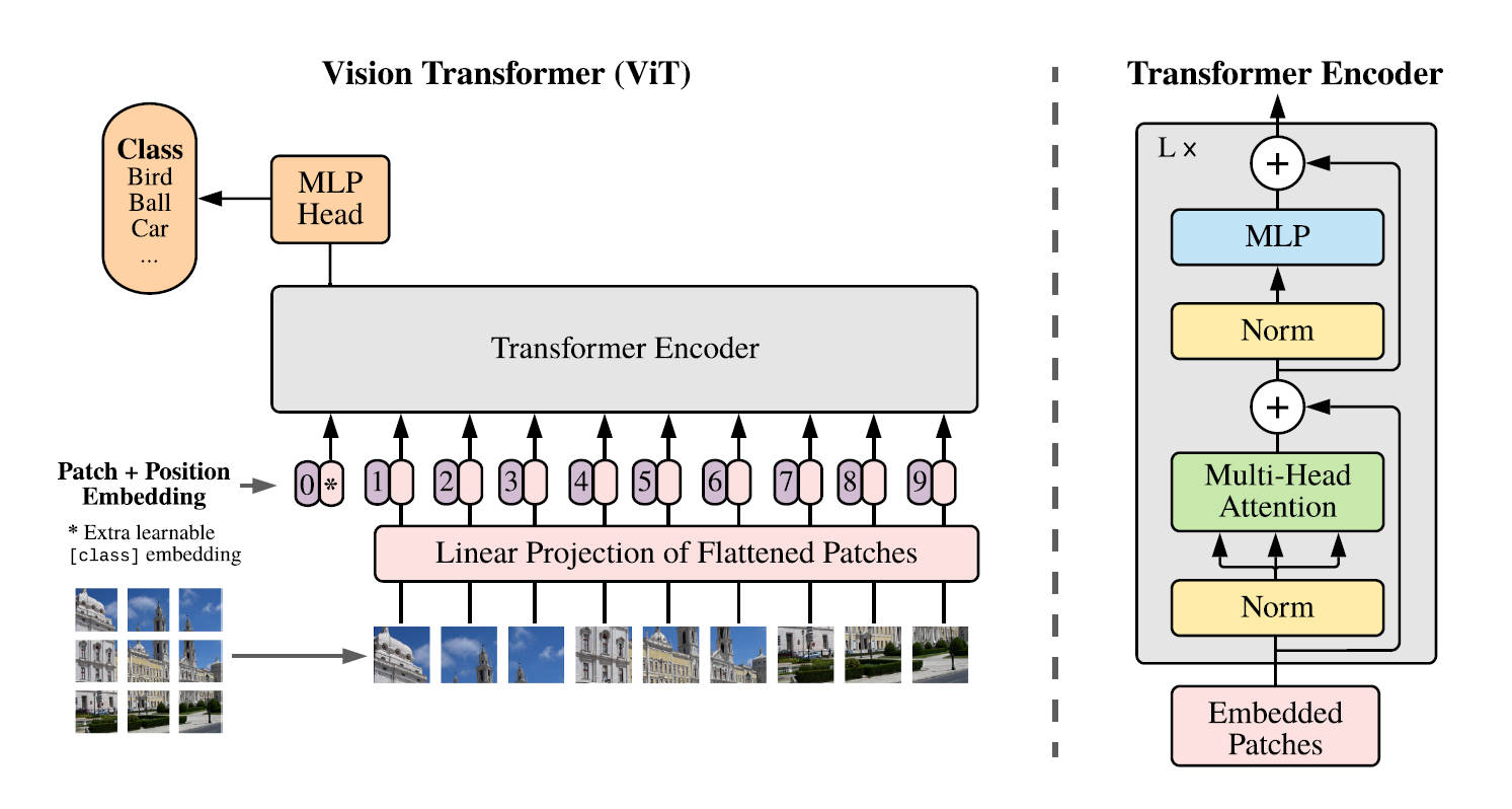
模型总览图如上,上一节实现的就是Embedded Patches模块。论文中的数据是在大数据集的情况下进行训练的,但是作为学习这篇论文,大数据集训练对个人电脑还是十分困难的,所以选择MNIST数据集进行训练也是可以的,MNIST是单通道的数据,不用分开多个通道拼接,只需要划分patch然后拉成向量就可以了,然后根据模型图,ViT是只有编码器的,而且也没有Feed-Forward Network层,替换成MLP层进行分类,所以实现的Transformer只有一个Encoder层,还有一个分类头,然后叠加L层。EncodeLayer是上一篇学习周报的Transformer代码中的EncodeLayer。
python
import torch.optim as optim
from process import *
from transformer.model import *


class Transformer(nn.Module):
    def __init__(self, num_classes=10, d_model=49, num_heads=7, num_layers=4,
                 d_ff=196, max_seq_length=17, dropout=0.1):
        super().__init__()

        # 编码器层
        self.encoder_layers = nn.ModuleList([
            EncoderLayer(d_model, num_heads, d_ff, dropout) for _ in range(num_layers)
        ])

        # 分类头
        self.classifier = nn.Sequential(
            nn.LayerNorm(d_model),
            nn.Linear(d_model, num_classes)
        )

        self.dropout = nn.Dropout(dropout)

    def forward(self, x):
        # 编码器
        for enc_layer in self.encoder_layers:
            x = enc_layer(x, mask=None)

        # 使用CLS token进行分类
        cls_output = x[:, 0]  # 取第一个token (CLS token)

        # 分类
        output = self.classifier(cls_output)
        return output


# 训练函数
def train():
    # 初始化模型
    model = Transformer(
        num_classes=10,  # MNIST有10个类别
        d_model=49,
        num_heads=7,  # 49/7=7
        num_layers=4,
        d_ff=196,  # 4 * d_model
        max_seq_length=17  # CLS + 16个patch
    )

    # 优化器和损失函数
    optimizer = optim.Adam(model.parameters(), lr=0.001)
    criterion = nn.CrossEntropyLoss()

    # 训练参数
    num_epochs = 10
    device = torch.device('cuda' if torch.cuda.is_available() else 'cpu')
    model.to(device)

    print(f"使用设备: {device}")
    print(f"模型参数量: {sum(p.numel() for p in model.parameters()):,}")

    # 训练循环
    model.train()
    for epoch in range(num_epochs):
        total_loss = 0
        correct = 0
        total = 0

        for batch_idx in range(len(train_patches)):
            patches = train_patches[batch_idx]
            labels = train_labels[batch_idx]

            # 移动到设备
            patches, labels = patches.to(device), labels.to(device)

            # 前向传播
            optimizer.zero_grad()
            outputs = model(patches)
            loss = criterion(outputs, labels)

            # 反向传播
            loss.backward()
            optimizer.step()

            # 统计
            total_loss += loss.item()
            _, predicted = outputs.max(1)
            total += labels.size(0)
            correct += predicted.eq(labels).sum().item()

        accuracy = 100. * correct / total
        print(f'Epoch {epoch + 1} completed. Loss: {total_loss / len(train_patches):.4f}, Accuracy: {accuracy:.2f}%')

    return model


def test(model, test_patches, test_labels):
    """测试函数"""
    device = torch.device('cuda' if torch.cuda.is_available() else 'cpu')
    model.to(device)
    model.eval()

    correct = 0
    total = 0
    test_loss = 0
    criterion = nn.CrossEntropyLoss()

    print("\n开始测试...")
    with torch.no_grad():
        for batch_idx in range(len(test_patches)):
            patches = test_patches[batch_idx]
            labels = test_labels[batch_idx]

            # 移动到设备
            patches, labels = patches.to(device), labels.to(device)

            # 前向传播
            outputs = model(patches)
            loss = criterion(outputs, labels)

            # 统计
            test_loss += loss.item()
            _, predicted = outputs.max(1)
            total += labels.size(0)
            correct += predicted.eq(labels).sum().item()

    avg_test_loss = test_loss / len(test_patches)
    test_accuracy = 100. * correct / total

    print(f"\n测试结果:")
    print(f"测试损失: {avg_test_loss:.4f}")
    print(f"测试准确率: {test_accuracy:.2f}%")
    print(f"正确样本数: {correct}/{total}")

    return test_accuracy


if "__main__" == __name__:
    model = train()
    test(model, test_patches, test_labels)
1.3 论文
ViT的论文证明了纯Transformer结构在CV方面效果也是不错的,而且在大数据样本预训练的情况下,效果相比神经网络更好,训练更便宜。Transformer想真正应用到CV方面,还需要对图片特征做近似,不能把整个图片的像素作为token进行输入,现在的检测、识别图片像素值都比较高,如果把所有的像素作为输入,那序列的长度就会很长很长,自注意力机制会很久。所以需要做一些近似,拿一个小窗口或者或者对一些稀疏的点做注意力。
1.4 优缺点
ViT的训练更快,但是起效又需要大数据集,在中小型数据集上是低于神经网络模型的,因为缺少一些图片平移和特征在图片上相邻这些归纳偏置,所以会低一点。ViT的数据集十分的大,显得计算快的优点也没那么快了。Transformer在后面也用于了CV的其他领域,如:目标检测等;
1.5 对比
python
import torch
from torch import nn, optim
from torch.utils.data import DataLoader, Dataset, random_split
import numpy as np
import os

from torchvision import transforms


class MyData(Dataset):
    def __init__(self, path, data_name, lable_name, transform=None):
        super().__init__()
        self.path = path
        self.transform = transform
        self.data, self.label = self.load(data_name, lable_name)

    def __len__(self):
        return len(self.data)

    def __getitem__(self, idx):
        img = self.data[idx]
        label = int(self.label[idx])
        if self.transform is not None:
            img = self.transform(img)
        return img, label

    def load(self, data_name, label_name):
        with open(os.path.join(self.path, label_name), 'rb') as f:
            y = np.frombuffer(f.read(), np.uint8, offset=8)
        with open(os.path.join(self.path, data_name), 'rb') as f:
            x = np.frombuffer(f.read(), np.uint8, offset=16).reshape(len(y), 28, 28)
        return np.array(x, copy=True), np.array(y, copy=True)


class BasicBlock(nn.Module):
    """基础残差块,用于ResNet-18/34"""
    expansion = 1

    def __init__(self, in_channels, out_channels, stride=1):
        super(BasicBlock, self).__init__()
        # 主路径
        self.conv1 = nn.Conv2d(in_channels, out_channels, kernel_size=3,
                               stride=stride, padding=1, bias=False)
        self.bn1 = nn.BatchNorm2d(out_channels)
        self.relu = nn.ReLU(inplace=True)
        self.conv2 = nn.Conv2d(out_channels, out_channels, kernel_size=3,
                               stride=1, padding=1, bias=False)
        self.bn2 = nn.BatchNorm2d(out_channels)
        # 短路连接
        self.shortcut = nn.Sequential()
        if stride != 1 or in_channels != out_channels:
            self.shortcut = nn.Sequential(
                nn.Conv2d(in_channels, out_channels, kernel_size=1,
                          stride=stride, bias=False),
                nn.BatchNorm2d(out_channels)
            )

    def forward(self, x):
        identity = x
        out = self.conv1(x)
        out = self.bn1(out)
        out = self.relu(out)
        out = self.conv2(out)
        out = self.bn2(out)
        identity = self.shortcut(identity)
        out += identity
        out = self.relu(out)

        return out


class ResNet(nn.Module):
    def __init__(self, num_classes=10):
        super().__init__()

        self.in_channels = 64
        self.conv1 = nn.Conv2d(1, 64, kernel_size=3, stride=1, padding=1, bias=False)
        self.bn1 = nn.BatchNorm2d(64)
        self.relu = nn.ReLU(inplace=True)

        # 3个残差层
        self.layer1 = self._make_layer(64, 2, stride=1)  # 2个块
        self.layer2 = self._make_layer(128, 2, stride=2)  # 2个块
        self.layer3 = self._make_layer(256, 2, stride=2)  # 2个块

        self.avgpool = nn.AdaptiveAvgPool2d((1, 1))
        self.fc = nn.Linear(256, num_classes)

    def _make_layer(self, out_channels, blocks, stride):
        layers = []
        layers.append(BasicBlock(self.in_channels, out_channels, stride))
        self.in_channels = out_channels

        for _ in range(1, blocks):
            layers.append(BasicBlock(self.in_channels, out_channels))

        return nn.Sequential(*layers)

    def forward(self, x):
        x = self.conv1(x)
        x = self.bn1(x)
        x = self.relu(x)

        x = self.layer1(x)
        x = self.layer2(x)
        x = self.layer3(x)

        x = self.avgpool(x)
        x = x.view(x.size(0), -1)
        x = self.fc(x)

        return x


def train(model, train_loader, criterion, optimizer, device, epochs=10):
    """
    训练模型
    """
    model.train()
    for epoch in range(epochs):
        running_loss = 0.0
        correct = 0
        total = 0

        for batch_idx, (data, target) in enumerate(train_loader):
            data, target = data.to(device), target.to(device)

            optimizer.zero_grad()
            output = model(data)
            loss = criterion(output, target)
            loss.backward()
            optimizer.step()

            running_loss += loss.item()
            _, predicted = output.max(1)
            total += target.size(0)
            correct += predicted.eq(target).sum().item()

        accuracy = 100. * correct / total
        avg_loss = running_loss / len(train_loader)

        print(f'Epoch {epoch + 1}: Loss: {avg_loss:.4f} | Accuracy: {accuracy:.2f}%')


def test(model, test_loader, criterion, device):
    """
    测试模型
    """
    model.eval()
    test_loss = 0
    correct = 0
    total = 0

    with torch.no_grad():
        for data, target in test_loader:
            data, target = data.to(device), target.to(device)
            output = model(data)
            loss = criterion(output, target)

            test_loss += loss.item()
            _, predicted = output.max(1)
            total += target.size(0)
            correct += predicted.eq(target).sum().item()

    test_loss /= len(test_loader)
    accuracy = 100. * correct / total

    print(f'Average Loss: {test_loss:.4f} | Accuracy: {accuracy:.2f}%')

    return test_loss, accuracy


def main():
    device = torch.device("cuda" if torch.cuda.is_available() else "cpu")

    # 数据加载器参数
    batch_size = 10

    # 加载数据集
    data = MyData('../dataset/MNIST/raw/',
                   'train-images-idx3-ubyte',
                   'train-labels-idx1-ubyte',
                   transform=transforms.ToTensor())

    # 分割数据集
    train_size = int(0.8 * len(data))
    test_size = len(data) - train_size
    train_dataset, test_dataset = random_split(data, [train_size, test_size])

    # 创建数据加载器
    train_loader = DataLoader(train_dataset, batch_size=batch_size,
                              shuffle=True)
    test_loader = DataLoader(test_dataset, batch_size=batch_size,
                             shuffle=False)

    # 初始化模型
    model = ResNet(num_classes=10).to(device)

    # 定义损失函数和优化器
    criterion = nn.CrossEntropyLoss()
    optimizer = optim.Adam(model.parameters(), lr=0.001, weight_decay=1e-4)

    print("开始训练...")
    print(f"训练集大小: {len(train_dataset)}")
    print(f"测试集大小: {len(test_dataset)}")

    train(model, train_loader, criterion, optimizer, device, epochs=10)

    test_loss, accuracy = test(model, test_loader, criterion, device)
    print(f"Loss: {test_loss:.4f}, Accuracy: {accuracy:.2f}%")


if __name__ == "__main__":
    main()
以上是一个resnet10,准确率达到了98.73%,而ViT训练了10轮只有95%左右,所以通过对比发现在小数据集上,确实是神经网络的方法比transformer效率更高。
总结
本周学习了ViT,ViT在大数据上训练更快,模型效果经过大数据训练后的模型应用到中小型数据集上的效果比神经网络更好。对架构有了一些简单的理解,下周将对Swin-Transformer和MAE论文进行学习。