Python实现手写数字识别

手写数字识别（MNIST 数据集）

最经典、最有代表性的项目之一。

项目目标：让机器学习模型识别手写数字图片（0-9），判断图片上写的是什么数字。
数据集：MNIST（Mixed National Institute of Standards and Technology）

共 70,000 张灰度图片（28×28 像素）

60,000 张训练图片

10,000 张测试图片

每张图片只包含一个手写数字

python 复制代码

# 在环境里下载tensorflow，里面包含这个数据集
pip install numpy matplotlib tensorflow

代码以及结果如下

导入库

py 复制代码

# 导入库
import numpy as np # numpy库，提供多维数组对象
import matplotlib.pyplot as plt #Matplotlib库，用于绘画
from tensorflow.keras.datasets import mnist #TensorFlow 的 Keras 模块 --- MNIST 数据集
from tensorflow.keras.models import Sequential #Keras 模型类型
from tensorflow.keras.layers import Dense, Flatten #Keras 神经网络层，Dense（全连接层），Flatten（展平层）
from tensorflow.keras.utils import to_categorical #Keras 工具函数

解析

将整个库导入并起别名import ... as ...

py 复制代码

import numpy as np # numpy库，提供多维数组对象

py 复制代码

import matplotlib.pyplot as plt #Matplotlib库，用于绘画

从库中导入部分模块或函数from ... import ...

py 复制代码

from tensorflow.keras.models import Sequential #Keras 模型类型，只导入 Sequential 这个类

py 复制代码

from tensorflow.keras.layers import Dense, Flatten #Keras 神经网络层，Dense（全连接层），Flatten（展平层）从层模块中取出 Dense、Flatten 两个常用层

py 复制代码

from tensorflow.keras.utils import to_categorical #Keras 工具函数，从工具模块中取出标签转化函数

加载数据集

python 复制代码

# 直接从 Keras 加载 MNIST 数据集
(features_train, label_train), (features_test, label_test) = mnist.load_data()

print("训练集形状:", features_train.shape)
print("测试集形状:", features_test.shape)

分析

python 复制代码

# 直接从 Keras 加载 MNIST 数据集
print("我拿到的数据：",mnist.load_data())

可以看到获取到了两个元组数据，于是我们用(features_train, label_train), (features_test, label_test) 来获取数据，一个是训练数据，一个是测试数据
而每个元组里又有两个numpy.ndarrays数据array(feature)和arrary(label)

python 复制代码

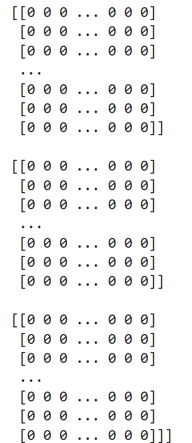
print(features_train)
print(label_train)
print("features_train 类型:", type(features_train))
print("label_train 类型:", type(label_train))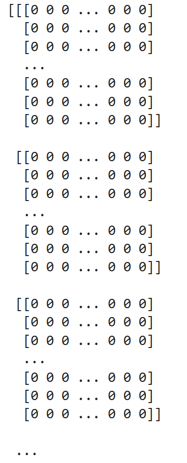

python 复制代码

# 直接从 Keras 加载 MNIST 数据集
(features_train, label_train), (features_test, label_test) = mnist.load_data()

print("训练集形状:", features_train.shape)
print("features_train 类型:", type(features_train))
print("features_train 元素类型:", features_train.dtype)
print(features_train[1])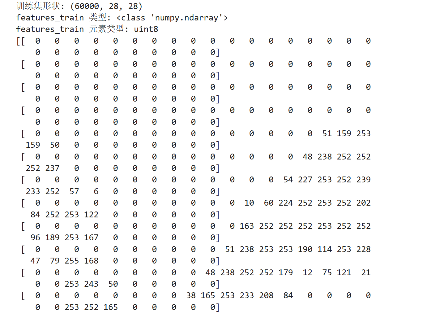

可以看到features_train里是28*28的int8整型矩阵，一共有6000个

py 复制代码

# 直接从 Keras 加载 MNIST 数据集
(features_train, label_train), (features_test, label_test) = mnist.load_data()

# print("训练集形状:", features_train.shape)
# print("features_train 类型:", type(features_train))
# print("features_train 元素类型:", features_train.dtype)
# print(features_train[1])

print("训练集形状:", label_train.shape)
print("label_train 类型:", type(label_train))
print("label_train 元素类型:", label_train.dtype)
print(label_train[:10])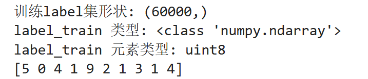

可以看到label_train里是6000个int8型的数字，也就是0-9的标签

数据可视化

看一看这里的灰度图片

python 复制代码

plt.figure(figsize=(8,3))
for i in range(10):
    plt.subplot(2,5,i+1)
    plt.imshow(features_train[i], cmap='gray')
    plt.title(f"Label: {label[i]}")
    plt.axis('off')
plt.show()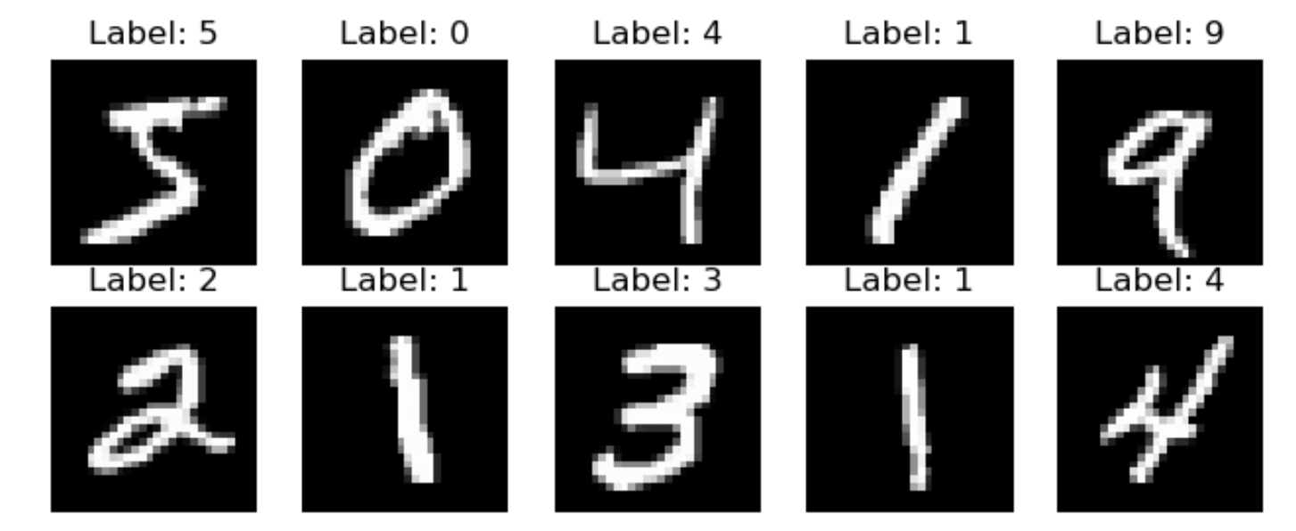

python 复制代码

# 首先创建一个画布,大小为 8 英寸 × 3 英寸
plt.figure(figsize=(8,3))

python 复制代码

# 放10张图片，编号从 0 到 9
for i in range(10):
    plt.subplot(2,5,i+1) #把画布划分成 2 行 5 列 的小格子（共 10 个小图）
    plt.imshow(features_train[i], cmap='gray') #用灰度图颜色显示
    plt.title(f "Label: {label[i]}") #动态显示标签：Label: 5、Label: 3
    plt.axis('off') #去掉坐标轴

py 复制代码

plt.show() #最后统一显示图像窗口

数据预处理

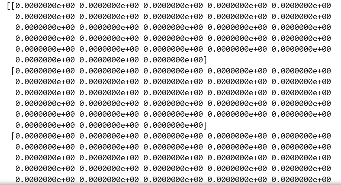
归一化

python 复制代码

features_train = features_train.astype("float32") / 255
features_test = features_test.astype("float32") / 255

把图像的数据类型从 整数型（uint8） 转换为 浮点型（float32）

MNIST 数据原始是 0～255 的整数（代表像素灰度值）

机器学习中的模型计算一般使用 浮点数，这样可以进行更精确的梯度计算。
归一化

把像素值 归一化（Normalization） 到 0～1 之间。

因为每个像素的灰度值原本是0-255，归一化就变成0.0-0.1。这样能让训练更加稳定，不会因为数值太大导致梯度爆炸或收敛困难。

独热编码

标签是整数形式，但是神经网络在做分类时，最后一层会输出一个概率分布。

为了跟这个概率分布进行比较，我们需要把原本的标签（一个数字）也转成相同形状的概率向量 。

这就是 独热编码（One-hot encoding）。

to_categorical() 的功能是把标签数字转成这种「向量表示」

原始标签	One-hot 编码
0	[1,0,0,0,0,0,0,0,0,0]
1	[0,1,0,0,0,0,0,0,0,0]
5	[0,0,0,0,0,1,0,0,0,0]
9	[0,0,0,0,0,0,0,0,0,1]

python 复制代码

label_train = to_categorical(label_train)
label_test = to_categorical(label_test)

模型训练

构建顺序模型

python 复制代码

model = Sequential([
    Flatten(input_shape=(28,28)),   # 把28x28二维图展平成784维向量
    Dense(128, activation='relu'),  # 隐藏层：128个神经元
    Dense(10, activation='softmax') # 输出层：10类（数字0-9）
])

层	作用	说明
`Flatten(input_shape=(28,28))`	把图片摊平	MNIST 图片是 28×28 像素的二维数组，需要摊平成一维向量（784个数）才能输入全连接层
`Dense(128, activation='relu')`	全连接层（隐藏层）	有 128 个神经元，每个神经元都连接前一层的所有输入。`relu` 是一种激活函数（能让模型学习非线性关系）
`Dense(10, activation='softmax')`	输出层	因为我们有 10 个类别（数字 0--9），所以输出 10 个概率；`softmax` 把它们归一化为「总和 = 1」的概率分布

编译模型

python 复制代码

model.compile(
    optimizer='adam',                 # 优化算法
    loss='categorical_crossentropy',  # 分类损失函数
    metrics=['accuracy']              # 评估指标
)

参数	含义
`optimizer='adam'`	优化算法，用来更新权重（Adam 是一种自适应学习率算法，非常常用）
`loss='categorical_crossentropy'`	损失函数：衡量模型预测与真实标签之间的差距。适合「多分类 + one-hot 标签」的任务
`metrics=['accuracy']`	训练时除了损失，还要计算准确率（accuracy）方便观察模型效果

训练模型

python 复制代码

history = model.fit(
    feature_train, label_train,
    epochs=5,
    batch_size=128,
    validation_split=0.1
)

参数	说明
`feature_train, label_train`	训练数据与标签
`epochs=5`	整个训练集会被重复学习 5 次
`batch_size=128`	每次送入网络的样本数量（越大训练越快，但显存占用高）
`validation_split=0.1`	从训练集中拿出 10% 作为验证集，用来检测模型是否过拟合
`history`	保存训练过程中的损失、准确率等指标，方便后面画图分析

复制代码

输入：28x28灰度图
   ↓ Flatten
784维输入向量
   ↓ Dense(128, ReLU)
提取特征
   ↓ Dense(10, Softmax)
输出10个类别概率
   ↓
计算损失 → 优化器更新参数 → 重复多轮（epochs）

模型评估

python 复制代码

test_loss, test_acc = model.evaluate(feature_test, label_test)
#让模型在测试集上跑一遍，不训练，只评估
print("测试集准确率:", test_acc)

输出	含义
`test_loss`	模型在测试集上的损失值（越小越好）
`test_acc`	模型在测试集上的准确率（accuracy）

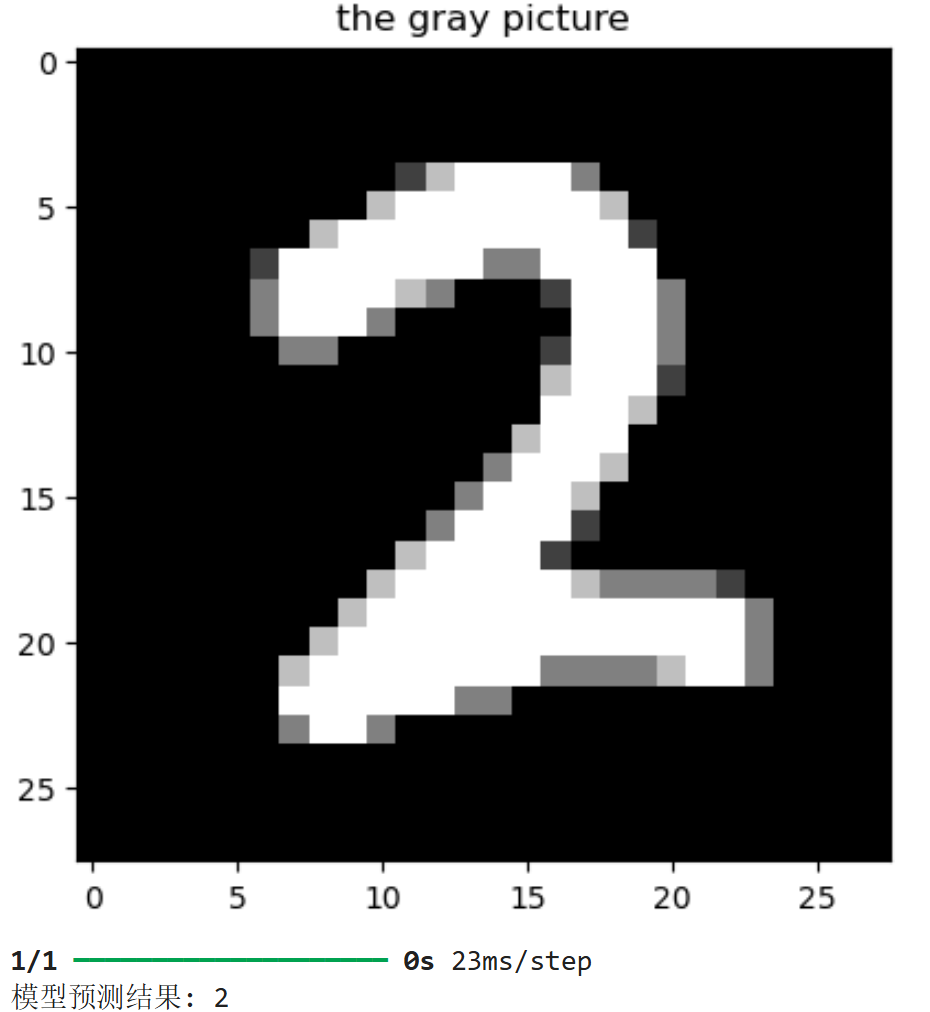
测试单张图片

python 复制代码

#展示一张图片
index = np.random.randint(0, 10000)#随机生成一个测试样本的索引（0 到 9999 之间）
plt.imshow(feature_test[index], cmap='gray')
plt.title("the gray picture")
plt.show()

python 复制代码

# 模型预测部分
pred = model.predict(feature_test[index].reshape(1,28,28))
print("模型预测结果:", np.argmax(pred))

操作	说明
`feature_test[index]`	取出那张图片（形状是 `(28,28)`）
`.reshape(1,28,28)`	变形为模型能接受的输入 `(1,28,28)`，表示"1张图片"，因为模型要求输入是批量(batch) 形式
`model.predict(...)`	让模型输出预测结果（一个长度为 10 的数组，每个数代表对应数字的概率）

代码：顺序模型

py 复制代码

# 导入库
import numpy as np # numpy库，提供多维数组对象
import matplotlib.pyplot as plt #Matplotlib库，用于绘画
from tensorflow.keras.datasets import mnist #TensorFlow 的 Keras 模块 --- MNIST 数据集
from tensorflow.keras.models import Sequential #Keras 模型类型
from tensorflow.keras.layers import Dense, Flatten #Keras 神经网络层，Dense（全连接层），Flatten（展平层）
from tensorflow.keras.utils import to_categorical #Keras 工具函数

# 直接从 Keras 加载 MNIST 数据集
(features_train, label_train), (features_test, label_test) = mnist.load_data()

print("训练集形状:", features_train.shape)
print("测试集形状:", features_test.shape)

#数据可视化
plt.figure(figsize=(8,3))
for i in range(10):
    plt.subplot(2,5,i+1)
    plt.imshow(features_train[i], cmap='gray')
    plt.title(f"Label: {label[i]}")
    plt.axis('off')
plt.show()

#构建顺序模型
model = Sequential([
    Flatten(input_shape=(28,28)),   # 把28x28二维图展平成784维向量
    Dense(128, activation='relu'),  # 隐藏层：128个神经元
    Dense(10, activation='softmax') # 输出层：10类（数字0-9）
])

#编译模型
model.compile(
    optimizer='adam',                 # 优化算法
    loss='categorical_crossentropy',  # 分类损失函数
    metrics=['accuracy']              # 评估指标
)

#训练模型
history = model.fit(
    feature_train, label_train,
    epochs=5,
    batch_size=128,
    validation_split=0.1
)

#模型评估
test_loss, test_acc = model.evaluate(feature_test, label_test)
#让模型在测试集上跑一遍，不训练，只评估
print("测试集准确率:", test_acc)

#展示一张图片
index = np.random.randint(0, 10000)#随机生成一个测试样本的索引（0 到 9999 之间）
plt.imshow(feature_test[index], cmap='gray')
plt.title("the gray picture")
plt.show()

# 模型预测部分
pred = model.predict(feature_test[index].reshape(1,28,28))
print("模型预测结果:", np.argmax(pred))

代码：CNN卷积神经网络

py 复制代码

# 导入库
import numpy as np
import matplotlib.pyplot as plt
from tensorflow.keras.datasets import mnist
from tensorflow.keras.models import Sequential
from tensorflow.keras.layers import Conv2D, MaxPooling2D, Flatten, Dense, Dropout
from tensorflow.keras.utils import to_categorical

#加载数据
# 直接从 Keras 加载 MNIST 数据集
(features_train, label_train), (features_test, label_train) = mnist.load_data()

print("训练集形状:", features_train.shape)
print("测试集形状:", features_test.shape)

#数据预处理
# CNN 需要输入三维数据 (height, width, channels)，而 MNIST 是灰度图（只有 1 个通道）
# 调整维度 (60000, 28, 28, 1)
features_train = features_train.reshape(-1, 28, 28, 1).astype("float32") / 255
features_test = features_test.reshape(-1, 28, 28, 1).astype("float32") / 255

# One-hot 编码
label_train = to_categorical(label_train, 10)
label_train = to_categorical(label_train, 10)

#构建CNN模型
model = Sequential([
    # 卷积层1：32个卷积核 3x3
    Conv2D(32, kernel_size=(3,3), activation='relu', input_shape=(28,28,1)),
    MaxPooling2D(pool_size=(2,2)),

    # 卷积层2：64个卷积核 3x3
    Conv2D(64, kernel_size=(3,3), activation='relu'),
    MaxPooling2D(pool_size=(2,2)),

    Flatten(),                  # 展平为一维
    Dropout(0.5),               # 防止过拟合
    Dense(128, activation='relu'),
    Dense(10, activation='softmax')  # 输出层（10类）
])

#编译模型
model.compile(
    optimizer='adam',
    loss='categorical_crossentropy',
    metrics=['accuracy']
)

#训练模型
history = model.fit(
    features_train, test_train,
    epochs=5,
    batch_size=128,
    validation_split=0.1,
    verbose=2
)

#评估模型
test_loss, test_acc = model.evaluate(features_test, label_test)
print("测试集准确率:", round(test_acc * 100, 2), "%")

#随机预测展示
index = np.random.randint(0, len(x_test))
plt.imshow(x_test[index].reshape(28,28), cmap='gray')
plt.title("图片预览")
plt.axis('off')
plt.show()


pred = model.predict(x_test[index].reshape(1,28,28,1))
print("模型预测结果:", np.argmax(pred))