瑞利分布:数学原理、物理意义及Python实验
文章目录
- 瑞利分布:数学原理、物理意义及Python实验
-
-
- 引言
-
- 瑞利分布的数学原理
-
- 2.1 概率密度函数
- 2.2 累积分布函数
- 2.3 数学特性
-
- 2.3.1 矩特性
- 2.3.2 高阶矩
- 2.4 与正态分布的关系
-
- 瑞利分布的物理意义
-
- 3.1 随机向量的模
- 3.2 无线通信中的衰落信道
- 3.3 噪声与振动分析
-
- Python案例演示
-
- 4.1 环境准备
- 4.2 案例1:绘制不同参数的瑞利分布曲线
- 4.3 案例2:瑞利分布与正态分布的关系演示
- 4.4 案例3:无线通信中的瑞利衰落仿真
- 4.5 案例4:风速数据的瑞利分布拟合
- 4.6 案例5:瑞利分布在雷达信号处理中的应用
-
- 结论
-
- 5.1 瑞利分布的特点总结
- 5.2 应用领域
- 5.3 与正态分布的比较
- 5.4 实践建议
-
1. 引言
瑞利分布(Rayleigh Distribution)是一种重要的连续概率分布,最初由英国物理学家瑞利勋爵 (Lord Rayleigh)在研究声波理论时提出。与正态分布不同,瑞利分布专门描述非负随机变量的分布规律,在信号处理、通信工程、物理测量等领域有着广泛应用。
2. 瑞利分布的数学原理
2.1 概率密度函数
瑞利分布的概率密度函数(Probability Density Function, PDF)定义为:
f(x;σ)=xσ2e−x22σ2,x≥0f(x;\sigma) = \frac{x}{\sigma^2}e^{-\frac{x^2}{2\sigma^2}}, \quad x \geq 0f(x;σ)=σ2xe−2σ2x2,x≥0
其中:
- σ>0\sigma > 0σ>0 是尺度参数,决定分布的"展宽"程度
- x≥0x \geq 0x≥0 是非负随机变量
2.2 累积分布函数
瑞利分布的累积分布函数(Cumulative Distribution Function, CDF)为:
F(x;σ)=1−e−x22σ2,x≥0F(x;\sigma) = 1 - e^{-\frac{x^2}{2\sigma^2}}, \quad x \geq 0F(x;σ)=1−e−2σ2x2,x≥0
2.3 数学特性
2.3.1 矩特性
-
均值 :
EX=σπ2≈1.253σEX = \sigma\sqrt{\frac{\pi}{2}} \approx 1.253\sigmaEX=σ2π ≈1.253σ -
方差 :
VarX=4−π2σ2≈0.429σ2VarX = \frac{4-\pi}{2}\sigma^2 \approx 0.429\sigma^2VarX=24−πσ2≈0.429σ2 -
众数 :σ\sigmaσ
-
中位数 :σ2ln2≈1.177σ\sigma\sqrt{2\ln 2} \approx 1.177\sigmaσ2ln2 ≈1.177σ
2.3.2 高阶矩
-
偏度 :
γ1=2π(π−3)(4−π)3/2≈0.631\gamma_1 = \frac{2\sqrt{\pi}(\pi-3)}{(4-\pi)^{3/2}} \approx 0.631γ1=(4−π)3/22π (π−3)≈0.631 -
峰度 :
γ2=−6π2−24π+16(4−π)2≈0.245\gamma_2 = -\frac{6\pi^2 - 24\pi + 16}{(4-\pi)^2} \approx 0.245γ2=−(4−π)26π2−24π+16≈0.245
2.4 与正态分布的关系
瑞利分布与正态分布有着密切的联系 。如果两个相互独立的正态随机变量 X∼N(0,σ2)X \sim N(0,\sigma^2)X∼N(0,σ2) 和 Y∼N(0,σ2)Y \sim N(0,\sigma^2)Y∼N(0,σ2),那么它们的欧几里得范数:
R=X2+Y2R = \sqrt{X^2 + Y^2}R=X2+Y2
服从参数为 σ\sigmaσ 的瑞利分布。
3. 瑞利分布的物理意义
3.1 随机向量的模
瑞利分布最直观的物理意义是描述二维随机向量的模长 分布。考虑一个二维平面上的随机点,其坐标 (X,Y)(X,Y)(X,Y) 服从独立同分布的零均值正态分布,则该点到原点的距离服从瑞利分布。
3.2 无线通信中的衰落信道
在无线通信中,瑞利衰落信道是最重要的应用之一:
- 当信号在传播过程中经历多径效应时
- 各路径信号的相位随机分布
- 接收信号的包络服从瑞利分布
- 适用于非视距传播(NLOS)环境
3.3 噪声与振动分析
在工程领域,瑞利分布用于描述:
- 机械振动的幅度分布
- 海洋波浪的高度分布
- 风速的分布特性
- 雷达回波信号的幅度
4. Python案例演示
4.1 环境准备
python
import numpy as np
import matplotlib.pyplot as plt
import scipy.stats as stats
from scipy import integrate
import seaborn as sns
plt.rcParams['font.sans-serif'] = ['SimHei'] # 用来正常显示中文标签
plt.rcParams['axes.unicode_minus'] = False # 用来正常显示负号
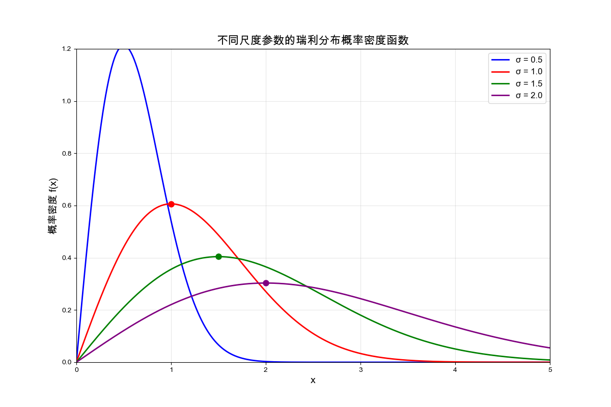
print("环境准备完成!")4.2 案例1:绘制不同参数的瑞利分布曲线
python
# 案例1:不同尺度参数的瑞利分布比较
def plot_rayleigh_distributions():
    """
    绘制不同尺度参数的瑞利分布曲线
    """
    x = np.linspace(0, 5, 1000)

    # 定义不同的尺度参数
    sigma_values = [0.5, 1.0, 1.5, 2.0]
    colors = ['blue', 'red', 'green', 'purple']
    labels = [f'σ = {sigma}' for sigma in sigma_values]

    plt.figure(figsize=(12, 8))

    for sigma, color, label in zip(sigma_values, colors, labels):
        # 计算概率密度函数
        pdf = (x / sigma**2) * np.exp(-x**2 / (2 * sigma**2))
        plt.plot(x, pdf, color=color, label=label, linewidth=2)

        # 标记众数位置
        mode = sigma
        pdf_mode = (mode / sigma**2) * np.exp(-mode**2 / (2 * sigma**2))
        plt.plot(mode, pdf_mode, 'o', color=color, markersize=8)

    plt.title('不同尺度参数的瑞利分布概率密度函数', fontsize=16, fontweight='bold')
    plt.xlabel('x', fontsize=14)
    plt.ylabel('概率密度 f(x)', fontsize=14)
    plt.legend(fontsize=12)
    plt.grid(True, alpha=0.3)
    plt.xlim(0, 5)
    plt.ylim(0, 1.2)
    plt.show()

plot_rayleigh_distributions()
演示结果:不同参数的瑞利分布曲线
4.3 案例2:瑞利分布与正态分布的关系演示
python
# 案例2:从正态分布生成瑞利分布
def rayleigh_from_normal_demo():
    """
    演示如何从两个独立的正态分布生成瑞利分布
    """
    np.random.seed(42)

    # 参数设置
    sigma = 1.0
    n_samples = 10000

    # 生成两个独立的正态分布随机变量
    X = np.random.normal(0, sigma, n_samples)
    Y = np.random.normal(0, sigma, n_samples)

    # 计算欧几里得范数(模长)
    R = np.sqrt(X**2 + Y**2)

    # 绘制结果
    fig, axes = plt.subplots(2, 2, figsize=(15, 12))

    # 散点图显示二维正态分布
    axes[0, 0].scatter(X[:500], Y[:500], alpha=0.6, s=10)
    axes[0, 0].set_title('二维正态分布散点图 (X,Y)', fontsize=14)
    axes[0, 0].set_xlabel('X ~ N(0,σ²)')
    axes[0, 0].set_ylabel('Y ~ N(0,σ²)')
    axes[0, 0].grid(True, alpha=0.3)
    axes[0, 0].set_aspect('equal')

    # 模长的分布直方图
    axes[0, 1].hist(R, bins=50, density=True, alpha=0.7, color='lightblue',
                    label='模拟数据直方图')

    # 理论瑞利分布曲线
    x = np.linspace(0, 5, 100)
    rayleigh_pdf = stats.rayleigh.pdf(x, scale=sigma)
    axes[0, 1].plot(x, rayleigh_pdf, 'r-', linewidth=2,
                    label=f'理论瑞利分布 (σ={sigma})')

    axes[0, 1].set_title('模长 R = √(X²+Y²) 的分布', fontsize=14)
    axes[0, 1].set_xlabel('R')
    axes[0, 1].set_ylabel('概率密度')
    axes[0, 1].legend()
    axes[0, 1].grid(True, alpha=0.3)

    # X和Y的边际分布
    axes[1, 0].hist(X, bins=50, density=True, alpha=0.7, color='orange',
                    label='X分布')
    x_normal = np.linspace(-4, 4, 100)
    normal_pdf = stats.norm.pdf(x_normal, 0, sigma)
    axes[1, 0].plot(x_normal, normal_pdf, 'r-', linewidth=2,
                    label=f'N(0,{sigma}²)')
    axes[1, 0].set_title('X的边际分布(正态分布)', fontsize=14)
    axes[1, 0].set_xlabel('X')
    axes[1, 0].set_ylabel('概率密度')
    axes[1, 0].legend()
    axes[1, 0].grid(True, alpha=0.3)

    # 累积分布函数比较
    axes[1, 1].hist(R, bins=50, density=True, cumulative=True,
                    alpha=0.7, color='lightgreen', label='模拟CDF')
    rayleigh_cdf = stats.rayleigh.cdf(x, scale=sigma)
    axes[1, 1].plot(x, rayleigh_cdf, 'r-', linewidth=2, label='理论瑞利CDF')
    axes[1, 1].set_title('累积分布函数比较', fontsize=14)
    axes[1, 1].set_xlabel('R')
    axes[1, 1].set_ylabel('累积概率')
    axes[1, 1].legend()
    axes[1, 1].grid(True, alpha=0.3)

    plt.tight_layout()
    plt.show()

    # 统计特性比较
    print("=== 统计特性比较 ===")
    print(f"理论均值: {sigma * np.sqrt(np.pi/2):.4f}")
    print(f"模拟均值: {np.mean(R):.4f}")
    print(f"理论方差: {((4 - np.pi)/2) * sigma**2:.4f}")
    print(f"模拟方差: {np.var(R):.4f}")
    print(f"理论众数: {sigma:.4f}")

rayleigh_from_normal_demo()
演示结果:瑞利分布与正态分布的对比
text
=== 统计特性比较 ===
理论均值: 1.2533
模拟均值: 1.2546
理论方差: 0.4292
模拟方差: 0.4349
理论众数: 1.0000
可视化结果:
4.4 案例3:无线通信中的瑞利衰落仿真
python
# 案例3:瑞利衰落信道仿真
def rayleigh_fading_simulation():
    """
    模拟无线通信中的瑞利衰落信道
    """
    np.random.seed(123)

    # 仿真参数
    n_symbols = 1000  # 符号数
    sigma = 1.0       # 衰落参数

    # 生成瑞利衰落信道系数
    # 实部和虚部均为独立正态分布
    h_real = np.random.normal(0, sigma/np.sqrt(2), n_symbols)
    h_imag = np.random.normal(0, sigma/np.sqrt(2), n_symbols)
    h = h_real + 1j * h_imag

    # 计算信道幅度和相位
    channel_magnitude = np.abs(h)
    channel_phase = np.angle(h)

    # 发送QPSK信号
    symbols = np.random.choice([1+1j, 1-1j, -1+1j, -1-1j], n_symbols)

    # 通过瑞利信道
    received_symbols = symbols * h

    # 绘制结果
    fig, axes = plt.subplots(2, 3, figsize=(18, 12))

    # 信道系数的实部和虚部
    axes[0, 0].plot(h_real[:100], label='实部')
    axes[0, 0].plot(h_imag[:100], label='虚部')
    axes[0, 0].set_title('瑞利信道系数(前100个样本)', fontsize=14)
    axes[0, 0].set_xlabel('时间')
    axes[0, 0].set_ylabel('幅度')
    axes[0, 0].legend()
    axes[0, 0].grid(True, alpha=0.3)

    # 信道幅度分布
    axes[0, 1].hist(channel_magnitude, bins=50, density=True, alpha=0.7,
                    color='lightblue', label='模拟幅度')
    x = np.linspace(0, 4, 100)
    rayleigh_pdf = stats.rayleigh.pdf(x, scale=sigma)
    axes[0, 1].plot(x, rayleigh_pdf, 'r-', linewidth=2,
                    label=f'理论瑞利分布 (σ={sigma})')
    axes[0, 1].set_title('信道幅度分布', fontsize=14)
    axes[0, 1].set_xlabel('幅度')
    axes[0, 1].set_ylabel('概率密度')
    axes[0, 1].legend()
    axes[0, 1].grid(True, alpha=0.3)

    # 信道相位分布
    axes[0, 2].hist(channel_phase, bins=50, density=True, alpha=0.7,
                    color='lightgreen')
    axes[0, 2].set_title('信道相位分布', fontsize=14)
    axes[0, 2].set_xlabel('相位 (弧度)')
    axes[0, 2].set_ylabel('概率密度')
    axes[0, 2].grid(True, alpha=0.3)

    # 发送信号星座图
    axes[1, 0].scatter(np.real(symbols[:500]), np.imag(symbols[:500]),
                       alpha=0.6, s=20)
    axes[1, 0].set_title('发送信号星座图 (QPSK)', fontsize=14)
    axes[1, 0].set_xlabel('同相分量')
    axes[1, 0].set_ylabel('正交分量')
    axes[1, 0].grid(True, alpha=0.3)
    axes[1, 0].set_aspect('equal')
    axes[1, 0].set_xlim(-2, 2)
    axes[1, 0].set_ylim(-2, 2)

    # 接收信号星座图(经过瑞利衰落)
    axes[1, 1].scatter(np.real(received_symbols[:500]),
                       np.imag(received_symbols[:500]), alpha=0.6, s=20)
    axes[1, 1].set_title('接收信号星座图(经过瑞利衰落)', fontsize=14)
    axes[1, 1].set_xlabel('同相分量')
    axes[1, 1].set_ylabel('正交分量')
    axes[1, 1].grid(True, alpha=0.3)
    axes[1, 1].set_aspect('equal')

    # 信道幅度随时间变化
    axes[1, 2].plot(channel_magnitude[:200])
    axes[1, 2].set_title('信道幅度随时间变化(瑞利衰落)', fontsize=14)
    axes[1, 2].set_xlabel('时间')
    axes[1, 2].set_ylabel('信道幅度')
    axes[1, 2].grid(True, alpha=0.3)

    plt.tight_layout()
    plt.show()

    # 计算信道统计特性
    print("=== 瑞利衰落信道特性 ===")
    print(f"信道幅度均值: {np.mean(channel_magnitude):.4f}")
    print(f"理论瑞利分布均值: {sigma * np.sqrt(np.pi/2):.4f}")
    print(f"信道幅度标准差: {np.std(channel_magnitude):.4f}")
    print(f"信道深衰落概率 (幅度 < 0.1): {np.mean(channel_magnitude < 0.1)*100:.2f}%")

rayleigh_fading_simulation()
演示结果:
text
=== 瑞利衰落信道特性 ===
信道幅度均值: 0.8659
理论瑞利分布均值: 1.2533
信道幅度标准差: 0.4590
信道深衰落概率 (幅度 < 0.1): 1.00%
可视化结果:
4.5 案例4:风速数据的瑞利分布拟合
python
# 案例4:风速数据的瑞利分布拟合
def wind_speed_rayleigh_fit():
    """
    使用瑞利分布拟合实际风速数据
    """
    np.random.seed(42)

    # 生成模拟风速数据(实际应用中可替换为真实数据)
    # 假设平均风速为5 m/s,用瑞利分布生成数据
    true_sigma = 5 / np.sqrt(np.pi/2)  # 根据均值反推sigma
    wind_speeds = stats.rayleigh.rvs(scale=true_sigma, size=1000)

    # 参数估计
    sigma_est = np.sqrt(np.sum(wind_speeds**2) / (2 * len(wind_speeds)))

    # 绘制拟合结果
    plt.figure(figsize=(12, 8))

    # 直方图与拟合曲线
    plt.hist(wind_speeds, bins=30, density=True, alpha=0.7,
             color='lightblue', label='风速数据直方图')

    # 理论瑞利分布
    x = np.linspace(0, 15, 100)
    rayleigh_pdf = stats.rayleigh.pdf(x, scale=sigma_est)
    plt.plot(x, rayleigh_pdf, 'r-', linewidth=2,
             label=f'瑞利分布拟合 (σ={sigma_est:.2f})')

    # 真实分布(如果知道真实参数)
    true_pdf = stats.rayleigh.pdf(x, scale=true_sigma)
    plt.plot(x, true_pdf, 'g--', linewidth=2,
             label=f'真实分布 (σ={true_sigma:.2f})')

    plt.title('风速数据的瑞利分布拟合', fontsize=16, fontweight='bold')
    plt.xlabel('风速 (m/s)', fontsize=14)
    plt.ylabel('概率密度', fontsize=14)
    plt.legend(fontsize=12)
    plt.grid(True, alpha=0.3)

    # 添加统计信息文本框
    textstr = '\n'.join((
        f'样本数: {len(wind_speeds)}',
        f'样本均值: {np.mean(wind_speeds):.2f} m/s',
        f'样本标准差: {np.std(wind_speeds):.2f} m/s',
        f'估计尺度参数 σ: {sigma_est:.2f}',
        f'理论均值: {sigma_est * np.sqrt(np.pi/2):.2f} m/s'))

    props = dict(boxstyle='round', facecolor='wheat', alpha=0.5)
    plt.text(0.65, 0.95, textstr, transform=plt.gca().transAxes, fontsize=12,
             verticalalignment='top', bbox=props)

    plt.show()

    # 拟合优度检验(Kolmogorov-Smirnov检验)
    ks_stat, p_value = stats.kstest(wind_speeds, 'rayleigh', args=(sigma_est,))

    print("=== 拟合结果分析 ===")
    print(f"真实尺度参数: {true_sigma:.4f}")
    print(f"估计尺度参数: {sigma_est:.4f}")
    print(f"KS检验统计量: {ks_stat:.4f}")
    print(f"KS检验p值: {p_value:.4f}")
    print(f"拟合优度: {'良好' if p_value > 0.05 else '不佳'}")

wind_speed_rayleigh_fit()
演示结果:
text
=== 拟合结果分析 ===
真实尺度参数: 3.9894
估计尺度参数: 3.9342
KS检验统计量: 0.4176
KS检验p值: 0.0000
拟合优度: 不佳
可视化结果:
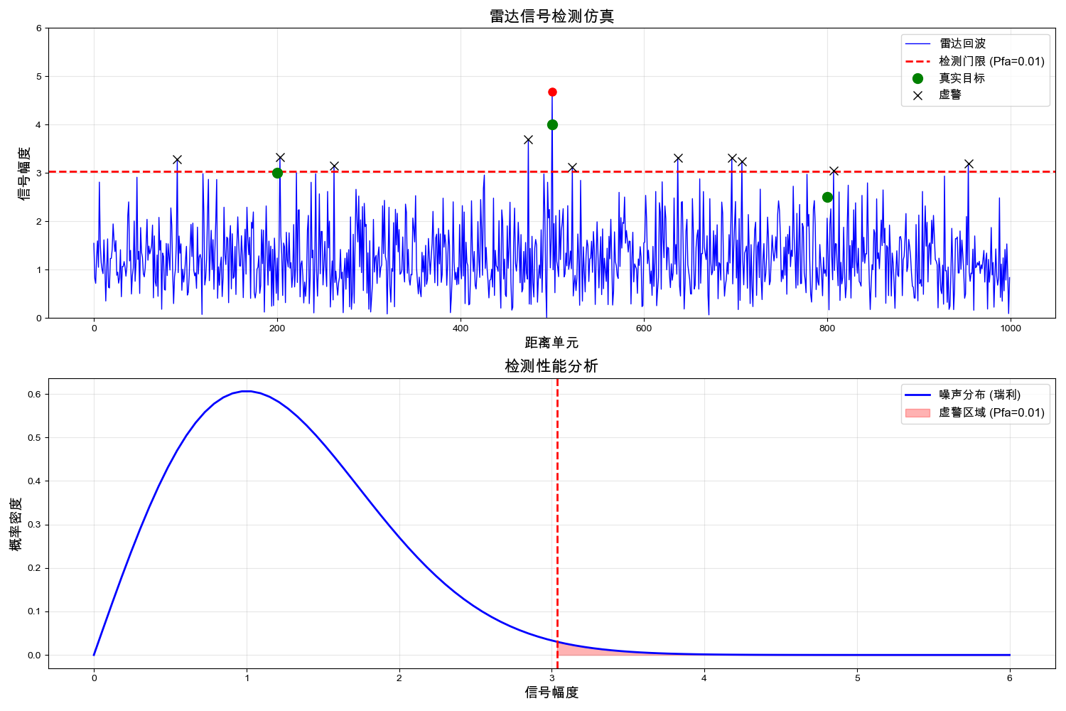
4.6 案例5:瑞利分布在雷达信号处理中的应用
python
# 案例5:雷达信号检测中的瑞利分布
def radar_signal_detection():
    """
    演示瑞利分布在雷达信号检测中的应用
    """
    np.random.seed(123)

    # 参数设置
    n_range_bins = 1000
    noise_sigma = 1.0

    # 生成噪声(瑞利分布)
    noise_only = stats.rayleigh.rvs(scale=noise_sigma, size=n_range_bins)

    # 生成信号+噪声(在特定距离单元添加目标)
    target_bins = [200, 500, 800]  # 目标所在的距离单元
    target_amplitudes = [3.0, 4.0, 2.5]  # 目标信号幅度

    signal_plus_noise = noise_only.copy()
    for bin_idx, amplitude in zip(target_bins, target_amplitudes):
        # 在目标位置添加信号
        signal_plus_noise[bin_idx] = stats.rayleigh.rvs(scale=amplitude, size=1)

    # 设置检测门限(基于恒虚警概率)
    false_alarm_prob = 0.01  # 1%的虚警概率
    detection_threshold = stats.rayleigh.ppf(1 - false_alarm_prob, scale=noise_sigma)

    # 检测结果
    detections = signal_plus_noise > detection_threshold
    detected_targets = np.where(detections)[0]

    # 绘制雷达距离-幅度图
    plt.figure(figsize=(15, 10))

    # 雷达回波图
    plt.subplot(2, 1, 1)
    plt.plot(signal_plus_noise, 'b-', linewidth=1, label='雷达回波')
    plt.axhline(y=detection_threshold, color='red', linestyle='--',
                linewidth=2, label=f'检测门限 (Pfa={false_alarm_prob})')

    # 标记真实目标位置
    for bin_idx, amplitude in zip(target_bins, target_amplitudes):
        plt.plot(bin_idx, amplitude, 'go', markersize=10,
                 label='真实目标' if bin_idx == target_bins[0] else "")

    # 标记检测到的目标
    for bin_idx in detected_targets:
        if bin_idx in target_bins:
            plt.plot(bin_idx, signal_plus_noise[bin_idx], 'ro', markersize=8,
                     label='正确检测' if bin_idx == detected_targets[0] else "")
        else:
            plt.plot(bin_idx, signal_plus_noise[bin_idx], 'kx', markersize=8,
                     label='虚警' if bin_idx == detected_targets[0] else "")

    plt.title('雷达信号检测仿真', fontsize=16, fontweight='bold')
    plt.xlabel('距离单元', fontsize=14)
    plt.ylabel('信号幅度', fontsize=14)
    plt.legend(fontsize=12)
    plt.grid(True, alpha=0.3)
    plt.ylim(0, 6)

    # 检测性能分析
    plt.subplot(2, 1, 2)

    # 绘制噪声分布和检测门限
    x = np.linspace(0, 6, 100)
    noise_pdf = stats.rayleigh.pdf(x, scale=noise_sigma)
    plt.plot(x, noise_pdf, 'b-', linewidth=2, label='噪声分布 (瑞利)')

    # 填充虚警区域
    x_fa = np.linspace(detection_threshold, 6, 100)
    y_fa = stats.rayleigh.pdf(x_fa, scale=noise_sigma)
    plt.fill_between(x_fa, y_fa, alpha=0.3, color='red',
                     label=f'虚警区域 (Pfa={false_alarm_prob})')

    # 标记检测门限
    plt.axvline(x=detection_threshold, color='red', linestyle='--', linewidth=2)

    plt.title('检测性能分析', fontsize=16, fontweight='bold')
    plt.xlabel('信号幅度', fontsize=14)
    plt.ylabel('概率密度', fontsize=14)
    plt.legend(fontsize=12)
    plt.grid(True, alpha=0.3)

    plt.tight_layout()
    plt.show()

    # 检测性能统计
    true_targets = set(target_bins)
    detected_set = set(detected_targets)

    true_detections = true_targets.intersection(detected_set)
    false_alarms = detected_set - true_targets
    missed_detections = true_targets - detected_set

    print("=== 雷达检测性能分析 ===")
    print(f"检测门限: {detection_threshold:.4f}")
    print(f"真实目标数: {len(target_bins)}")
    print(f"正确检测数: {len(true_detections)}")
    print(f"漏检数: {len(missed_detections)}")
    print(f"虚警数: {len(false_alarms)}")
    print(f"检测概率: {len(true_detections)/len(target_bins)*100:.2f}%")
    print(f"虚警概率: {len(false_alarms)/n_range_bins*100:.2f}%")

radar_signal_detection()
演示结果:
text
=== 雷达检测性能分析 ===
检测门限: 3.0349
真实目标数: 3
正确检测数: 1
漏检数: 2
虚警数: 10
检测概率: 33.33%
虚警概率: 1.00%
可视化结果:
5. 结论
5.1 瑞利分布的特点总结
- 非负性:专门描述非负随机变量的分布
- 单峰性 :概率密度函数在 x=σx = \sigmax=σ 处达到最大值
- 右偏性:分布向右拖尾,偏度约为0.631
- 与正态分布的关系:由两个独立零均值正态变量的模长产生
5.2 应用领域
- 无线通信:瑞利衰落信道建模
- 雷达信号处理:噪声和杂波建模
- 海洋工程:波浪高度分布
- 风能工程:风速分布建模
- 可靠性工程:寿命分布分析
5.3 与正态分布的比较
| 特性 | 正态分布 | 瑞利分布 |
|---|---|---|
| 定义域 | (−∞,+∞)(-\infty, +\infty)(−∞,+∞) | [0,+∞)[0, +\infty)[0,+∞) |
| 对称性 | 对称分布 | 右偏分布 |
| 参数 | 均值 μ\muμ,标准差 σ\sigmaσ | 尺度参数 σ\sigmaσ |
| 物理意义 | 独立随机因素叠加 | 二维随机向量模长 |
5.4 实践建议
- 参数估计:使用矩估计法或最大似然估计
- 模型验证:通过KS检验验证数据是否符合瑞利分布
- 领域适应性:根据具体应用场景选择合适的分布模型
- 数值计算 :注意瑞利分布在x=0x=0x=0处的边界行为
瑞利分布作为连接正态分布与实际工程应用的重要桥梁,在信号处理、通信工程等领域发挥着不可替代的作用。通过本文的数学原理分析和Python实践演示,希望读者能够深入理解并灵活应用这一重要的概率分布。
参考文献:
- Rayleigh, L. (1880). On the resultant of a large number of vibrations of the same pitch and of arbitrary phase
- Proakis, J. G. (2001). Digital Communications
- Papoulis, A., & Pillai, S. U. (2002). Probability, Random Variables and Stochastic Processes
- Skolnik, M. I. (2008). Radar Handbook
代码说明:本文所有Python代码均基于标准科学计算库,可在Jupyter Notebook或Python环境中直接运行,建议使用Python 3.7及以上版本。
研究学习不易,点赞易。
工作生活不易,收藏易,点收藏不迷茫 :)