9.8 贝塞尔曲线

文章目录

公式
贝塞尔曲线例子
德卡斯特柳算法

公式

贝塞尔曲线是鼎鼎有名哈，基本上只要学了点计算机都听过这个词，但是鲜有人知道它的公式与原理。贝塞尔曲线是分次数的，一次贝塞尔曲线就是一条直线，二次贝塞尔曲线由三个控制点决定，三次贝塞尔曲线最常用，由四个控制点决定，同理， n n n次贝塞尔曲线由 n + 1 n+1 n+1个控制点决定。其公式如下：
B ( t ) = ∑ i = 0 n ( n i ) ( 1 − t ) n − i t i P i , t ∈ [ 0 , 1 ] \bm{B}(t)=\sum_{i=0}^n{\binom{n}i(1-t)^{n-i}t^i}\bm{P}_i, ~~~~ t \in[0,1] B(t)=i=0∑n(in)(1−t)n−itiPi, t∈[0,1]

这和二项式定理长得很像啊：
( x + y ) n = ∑ i = 0 n ( n i ) x n − i y i (x+y)^n=\sum_{i=0}^n{\binom{n}ix^{n-i}y^i} (x+y)n=i=0∑n(in)xn−iyi

这是个定义在0到1之间的参数方程， t = 0 t=0 t=0就是第一个点， t = 1 t=1 t=1就是最后一个点。

贝塞尔曲线例子

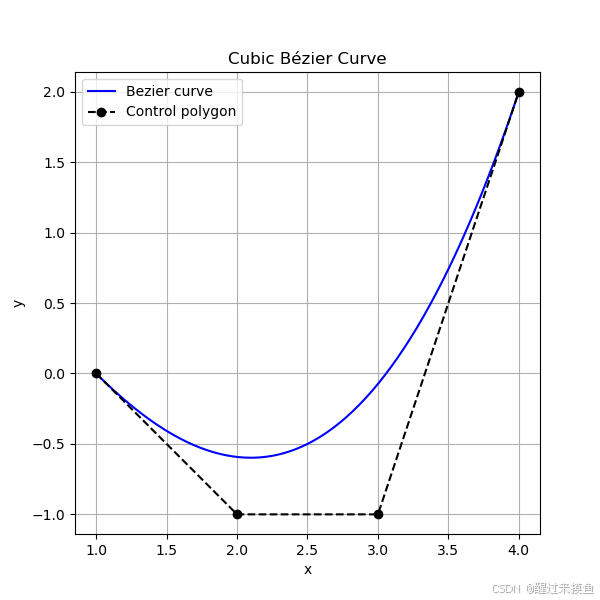
以下是直接根据公式，用Python画出来的贝塞尔曲线例子：

python 复制代码

import math

import numpy as np
import matplotlib.pyplot as plt

# 端点和控制点
P0 = np.array([1.0, 0.0])
P1 = np.array([2.0, -1.0])
P2 = np.array([3.0, -1.0])
P3 = np.array([4.0, 2.0])

def bezier(t, ctrl_pts):
    """
    通用 Bézier 曲线点计算
    参数
    ----
    t : float 或 ndarray，取值范围 [0, 1]
    ctrl_pts : ndarray，形状为 (m, d)
               m 为控制点数，d 为维度（2D、3D 等）
    返回
    ----
    point : ndarray，形状为 (d,)（若 t 为标量）或 (len(t), d)（若 t 为数组）
    """
    ctrl_pts = np.asarray(ctrl_pts, dtype=float)
    n = ctrl_pts.shape[0] - 1          # 曲线次数
    t = np.asarray(t, dtype=float)

    # 标量情况
    point = np.zeros(ctrl_pts.shape[1])
    for i in range(n + 1):
        point += math.comb(n, i) * (1 - t) ** (n - i) * t ** i * ctrl_pts[i]
    return point


if __name__ == '__main__':

    # 生成 t 参数
    t_vals = np.linspace(0, 1, 200)
    curve = np.array([bezier(t, [P0, P1, P2, P3]) for t in t_vals])
    # 绘图
    plt.figure(figsize=(6, 6))
    # 贝塞尔曲线
    plt.plot(curve[:, 0], curve[:, 1], 'b-', label='Bezier curve')
    # 控制多边形
    control_pts = np.vstack([P0, P1, P2, P3])
    plt.plot(control_pts[:, 0], control_pts[:, 1], 'k--', marker='o',
             label='Control polygon')
    plt.title('Cubic Bézier Curve')
    plt.xlabel('x')
    plt.ylabel('y')
    plt.axis('equal')
    plt.grid(True)
    plt.legend()
    plt.show()

效果图如下：

德卡斯特柳算法

我上面的代码，是直接按公式来的，就是下面这段python代码：

python 复制代码

def cubic_bezier(t, P0, P1, P2, P3):
    """计算参数 t（0~1）对应的三次贝塞尔曲线点"""
    return (1 - t) ** 3 * P0 + \
           3 * (1 - t) ** 2 * t * P1 + \
           3 * (1 - t) * t ** 2 * P2 + \
           t ** 3 * P3

直接这样算有什么不好？首先次数高了以后，浮点误差会放大，并且在兼容有理Bézier或带张力/偏移版的Bézier时，会非常繁琐。所以有了德卡斯特柳算法de Casteljau Algorithm 。

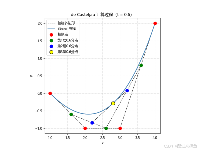
De Casteljau非常简单，其基本思想就是不断迭代降维，比如四个控制点的三次贝塞尔曲线，先转变为三个控制点的二次贝塞尔曲线，最后转变为两个控制点的直线。我用一张图解释就非常容易理解了，也更能诠释贝塞尔曲线的本质。

以 t = 0.1 t=0.1 t=0.1为例子，四个控制点用上面例子的数据。

数值计算过程就是：

第一次迭代：
P 0 ( 1 ) = ( 1 − t ) P 0 + t P 1 = 0.4 ( 1 , 0 ) + 0.6 ( 2 , − 1 ) = ( 1.6 , − 0.6 ) P 1 ( 1 ) = ( 1 − t ) P 1 + t P 2 = 0.4 ( 2 , − 1 ) + 0.6 ( 3 , − 1 ) = ( 2.6 , − 1.0 ) P 2 ( 1 ) = ( 1 − t ) P 2 + t P 3 = 0.4 ( 3 , − 1 ) + 0.6 ( 4 , 2 ) = ( 3.6 , 0.8 ) \begin{aligned} P_{0}^{(1)} &= (1-t)P_0 + tP_1 = 0.4\,(1,0)+0.6\,(2,-1) = (1.6,\,-0.6) \\[4pt] P_{1}^{(1)} &= (1-t)P_1 + tP_2 = 0.4\,(2,-1)+0.6\,(3,-1) = (2.6,\,-1.0) \\[4pt] P_{2}^{(1)} &= (1-t)P_2 + tP_3 = 0.4\,(3,-1)+0.6\,(4,2) = (3.6,\;0.8) \end{aligned} P0(1)P1(1)P2(1)=(1−t)P0+tP1=0.4(1,0)+0.6(2,−1)=(1.6,−0.6)=(1−t)P1+tP2=0.4(2,−1)+0.6(3,−1)=(2.6,−1.0)=(1−t)P2+tP3=0.4(3,−1)+0.6(4,2)=(3.6,0.8)

第二次迭代：
P 0 ( 2 ) = ( 1 − t ) P 0 ( 1 ) + t P 1 ( 1 ) = 0.4 ( 1.6 , − 0.6 ) + 0.6 ( 2.6 , − 1.0 ) = ( 2.2 , − 0.84 ) P 1 ( 2 ) = ( 1 − t ) P 1 ( 1 ) + t P 2 ( 1 ) = 0.4 ( 2.6 , − 1.0 ) + 0.6 ( 3.6 , 0.8 ) = ( 3.2 , 0.08 ) \begin{aligned} P_{0}^{(2)} &= (1-t)P_{0}^{(1)} + tP_{1}^{(1)} = 0.4\,(1.6,-0.6)+0.6\,(2.6,-1.0) \\ &= (2.2,\;-0.84) \\[4pt] P_{1}^{(2)} &= (1-t)P_{1}^{(1)} + tP_{2}^{(1)} = 0.4\,(2.6,-1.0)+0.6\,(3.6,0.8) \\ &= (3.2,\;0.08) \end{aligned} P0(2)P1(2)=(1−t)P0(1)+tP1(1)=0.4(1.6,−0.6)+0.6(2.6,−1.0)=(2.2,−0.84)=(1−t)P1(1)+tP2(1)=0.4(2.6,−1.0)+0.6(3.6,0.8)=(3.2,0.08)

第三次迭代：
P 0 ( 3 ) = ( 1 − t ) P 0 ( 2 ) + t P 1 ( 2 ) = 0.4 ( 2.2 , − 0.84 ) + 0.6 ( 3.2 , 0.08 ) = ( 2.8 , − 0.28 ) \begin{aligned} P_{0}^{(3)} &= (1-t)P_{0}^{(2)} + tP_{1}^{(2)} \\ &= 0.4\,(2.2,-0.84)+0.6\,(3.2,0.08) \\ &= (2.8,\;-0.28) \end{aligned} P0(3)=(1−t)P0(2)+tP1(2)=0.4(2.2,−0.84)+0.6(3.2,0.08)=(2.8,−0.28)

所以python实现也就很简单了：

python 复制代码

def de_casteljau(t, ctrl_pts):
    """
    de Casteljau 递归实现
    参数
    ----
    t : float  (0 ≤ t ≤ 1)
        曲线参数
    ctrl_pts : ndarray, shape (n+1, 2)
        控制点列表，n 为 Bézier 曲线次数
    返回
    ----
    point : ndarray, shape (2,)
        参数 t 对应的曲线点
    """
    pts = np.array(ctrl_pts, dtype=float)
    n = pts.shape[0] - 1          # 曲线次数
    # 逐层线性插值
    for r in range(1, n + 1):
        pts[:n - r + 1] = (1 - t) * pts[:n - r + 1] + t * pts[1:n - r + 2]
    return pts[0]