1、概要
我在gymnasium 的pendulum 环境上实现了PPO-clip 算法,并通过调节超参数 来探索超参数对训练过程 与训练结果的作用。
Pendulum环境:https://gymnasium.farama.org/environments/classic_control/pendulum/
PPO-clip:https://hrl.boyuai.com/chapter/2/ppo算法
2、代码
python
"""
======================================================================= # 训练配置
num_episodes = 500 # 训练回合数
batch_size = 2048 # 每次更新的样本数 (收集足够样本后才更新)
max_steps = 200 # 每回合最大步数 (与环境的 TimeLimit 一致)
# 保存和日志
model_save_path = 'models/ppo_pendulum.pth'
save_interval = 50 # 每隔多少回合保存一次模型
log_interval = 10 # 每隔多少回合输出一次日志
# 测试配置
test_episodes = 10 # 测试回合数
# ========== Weights & Biases 配置 ==========
use_wandb = True # 是否使用 wandb 进行实验跟踪
wandb_project = 'PPO-Pendulum' # wandb 项目名称
wandb_entity = None # wandb 用户名/团队名 (None 则使用默认)
wandb_run_name = None # 运行名称 (None 则自动生成)
wandb_tags = ['PPO', 'Pendulum', 'RL'] # 实验标签
wandb_notes = 'PPO-clip algorithm training on Pendulum-v1 environment' # 实验备注
# 设备配置
device = torch.device('cuda' if torch.cuda.is_available() else 'cpu')clip 算法训练 Gymnasium Pendulum 环境
================================================================================
算法说明:
PPO (Proximal Policy Optimization) 是一种策略梯度算法,通过限制策略更新的
幅度来保证训练的稳定性。PPO-clip 使用裁剪的目标函数来实现这一点。
使用方法:
1. 训练模式(不可视化,速度快):
python ppo_pendulum_continuous.py --mode train
2. 训练模式(可视化,查看动画):
python ppo_pendulum_continuous.py --mode train --visualize
3. 测试模式(可视化):
python ppo_pendulum_continuous.py --mode test --visualize
4. 测试模式(不可视化):
python ppo_pendulum_continuous.py --mode test
5. 测试模式(使用最终模型而非最佳模型):
python ppo_pendulum_continuous.py --mode test --use-final-model
6. 测试模式(使用自定义模型路径):
python ppo_pendulum_continuous.py --mode test --model-path models/PPO-Pendulum/exp1/best_model.pth
7. 自定义训练回合数:
python ppo_pendulum_continuous.py --mode train --episodes 1000
8. 自定义测试回合数:
python ppo_pendulum_continuous.py --mode test --test-episodes 20
9. 使用 Weights & Biases 进行实验跟踪 (推荐!):
python ppo_pendulum_continuous.py --mode train --wandb
10. 自定义实验名称和描述:
python ppo_pendulum_continuous.py --mode train --desc tuned --eps 0.2
# 自动生成: tuned_clip0.2_lr3e-4_gamma0.99_4000eps
11. 完全自定义实验配置:
python ppo_pendulum_continuous.py --mode train \
--project MyProject \
--experiment my-exp-v1 \
--eps 0.25 --actor-lr 1e-4 --episodes 2000 \
--wandb-tags experiment-1 tuning
12. 禁用 wandb:
python ppo_pendulum_continuous.py --mode train --no-wandb
测试模式说明:
- 默认加载最佳模型 (best_model.pth) - 训练过程中回报最高的模型
- 如果最佳模型不存在,自动回退到最终模型 (model.pth)
- 使用 --use-final-model 强制使用最终模型
- 使用 --model-path 指定任意模型文件路径
项目和实验命名规则:
- 项目名称(--project): 如 "PPO-Pendulum" (默认)
- 实验名称: 自动生成格式 "{描述}_clip{eps}_lr{actor_lr}_gamma{gamma}_{episodes}eps"
例如: baseline_clip0.3_lr3e-4_gamma0.99_4000eps
- 模型保存路径: models/{项目名称}/{实验名称}/model.pth
- 最佳模型路径: models/{项目名称}/{实验名称}/best_model.pth
- 训练曲线: models/{项目名称}/{实验名称}/training_curves.png
Weights & Biases 使用:
- 首次使用需要: pip install wandb && wandb login
- 详细教程请查看: wandb_tutorial.md
- 训练过程会实时上传到 wandb 网页,可在浏览器中查看
- 所有超参数、训练曲线、模型文件都会自动保存
输出说明:
- 训练过程会输出: 平均回报、Actor Loss、Critic Loss、步数等
- 训练结束会自动保存模型到 models/ppo_pendulum.pth
- 训练曲线会保存为 ppo_pendulum_training.png
- 测试会输出统计信息: 平均回报、标准差、最大最小值等
================================================================================
"""
import gymnasium as gym
import torch
import torch.nn.functional as F
import numpy as np
import matplotlib.pyplot as plt
from tqdm import tqdm
import argparse
import os
from collections import deque
import wandb # Weights & Biases 用于实验跟踪和可视化
# ==================== 超参数配置 ====================
class Config:
"""集中配置所有超参数"""
# ========== 项目和实验命名 ==========
project_name = 'PPO-Pendulum' # 项目名称 (用于目录结构和 wandb 项目)
experiment_name = None # 实验名称 (None 则自动生成,包含关键超参数)
experiment_desc = 'pendulum' # 实验描述 (简短说明,如 baseline, tuned, final)
# ========== 环境配置 ==========
# Pendulum-v1 环境说明:
# - 目标: 通过施加扭矩将倒立摆从随机位置摆到垂直向上
# - 观测空间: Box(3,) -> [cos(θ), sin(θ), 角速度]
# - 动作空间: Box(1,) -> 扭矩 τ ∈ [-2.0, 2.0]
# - 奖励函数: r = -(θ² + 0.1·θ̇² + 0.001·τ²), 范围约 [-16.27, 0]
# - 最大步数: 200 步 (通过 TimeLimit wrapper 实现)
env_name = 'Pendulum-v1'
render_mode = None # None (不渲染) 或 'human' (可视化) 或 'rgb_array'
env_g = 10.0 # 重力加速度 (默认 10.0, 真实值 9.81)
# ========== 网络配置 ==========
hidden_dim = 128 # 隐藏层神经元数量
# ========== PPO 超参数 ==========
actor_lr = 3e-4 # Actor 学习率
critic_lr = 1e-3 # Critic 学习率
gamma = 0.99 # 折扣因子 γ (用于计算未来奖励的衰减)
lmbda = 0.95 # GAE lambda (权衡偏差和方差)
eps = 0.2 # PPO clip 参数 ε (限制策略更新幅度)
epochs = 10 # 每批数据重复训练的轮数
# ========== 训练配置 ==========
num_episodes = 4000 # 训练回合数
batch_size = 2048 # 每次更新的样本数 (收集足够样本后才更新)
max_steps = 200 # 每回合最大步数 (与环境的 TimeLimit 一致)
# ========== 保存和日志配置 ==========
save_interval = 50 # 每隔多少回合保存一次模型
log_interval = 10 # 每隔多少回合输出一次日志
# ========== 测试配置 ==========
test_episodes = 10 # 测试回合数
# ========== Weights & Biases 配置 ==========
use_wandb = True # 是否使用 wandb 进行实验跟踪
wandb_entity = None # wandb 用户名/团队名 (None 则使用默认)
wandb_tags = ['PPO', 'Pendulum', 'RL'] # 实验标签
wandb_notes = 'PPO-clip algorithm training on Pendulum-v1 environment' # 实验备注
# ========== 设备配置 ==========
device = torch.device('cuda' if torch.cuda.is_available() else 'cpu')
def __init__(self):
"""初始化配置,生成实验名称和路径"""
# 如果未指定实验名称,则自动生成 (包含关键超参数)
if self.experiment_name is None:
self.experiment_name = self._generate_experiment_name()
# 生成模型保存路径: models/项目名称/实验名称/
self.model_save_dir = os.path.join('models', self.project_name, self.experiment_name)
self.model_save_path = os.path.join(self.model_save_dir, 'model.pth')
self.best_model_path = os.path.join(self.model_save_dir, 'best_model.pth')
# wandb 项目名称和运行名称
self.wandb_project = self.project_name
self.wandb_run_name = self.experiment_name
def _generate_experiment_name(self):
"""
自动生成实验名称,包含关键超参数
格式: {描述}_eps{eps}_lr{actor_lr}_gamma{gamma}_eps{num_episodes}
例如: baseline_eps0.3_lr3e-4_gamma0.99_4000eps
"""
# 格式化学习率 (3e-4 -> 3e-4)
lr_str = f"{self.actor_lr:.0e}".replace('-0', '-')
# 生成名称
name = (
f"{self.experiment_desc}_"
f"clip{self.eps}_"
f"lr{lr_str}_"
f"gamma{self.gamma}_"
f"{self.num_episodes}eps"
)
return name
def print_config(self):
"""打印配置信息"""
print("=" * 70)
print("配置信息")
print("=" * 70)
print(f"项目名称: {self.project_name}")
print(f"实验名称: {self.experiment_name}")
print(f"实验描述: {self.experiment_desc}")
print("-" * 70)
print(f"环境: {self.env_name}")
print(f"网络隐藏层: {self.hidden_dim}")
print(f"Actor 学习率: {self.actor_lr}")
print(f"Critic 学习率: {self.critic_lr}")
print(f"折扣因子 γ: {self.gamma}")
print(f"GAE λ: {self.lmbda}")
print(f"PPO clip ε: {self.eps}")
print(f"训练轮数/批: {self.epochs}")
print(f"训练回合数: {self.num_episodes}")
print(f"批大小: {self.batch_size}")
print("-" * 70)
print(f"模型保存目录: {self.model_save_dir}")
print(f"模型路径: {self.model_save_path}")
print(f"最佳模型路径: {self.best_model_path}")
print("-" * 70)
print(f"使用 wandb: {self.use_wandb}")
if self.use_wandb:
print(f"wandb 项目: {self.wandb_project}")
print(f"wandb 运行名称: {self.wandb_run_name}")
print(f"wandb 标签: {', '.join(self.wandb_tags)}")
print(f"设备: {self.device}")
print("=" * 70)
# ==================== 工具函数 ====================
def compute_advantage(gamma, lmbda, td_delta):
"""
计算 GAE (Generalized Advantage Estimation)
GAE 公式:
A^GAE(γ,λ)_t = Σ(γλ)^l * δ_t+l
其中 δ_t = r_t + γV(s_t+1) - V(s_t) 是 TD error
GAE 的优点:
- λ=0: 低方差但高偏差 (等价于 TD error)
- λ=1: 高方差但低偏差 (等价于 Monte Carlo)
- 0<λ<1: 在方差和偏差之间取得平衡
参数:
gamma: 折扣因子 γ
lmbda: GAE 参数 λ,控制偏差-方差权衡
td_delta: TD error 序列
返回:
advantage: 优势函数估计值
"""
td_delta = td_delta.detach().numpy()
advantage_list = []
advantage = 0.0
# 从后向前计算,利用递推关系: A_t = δ_t + γλA_t+1
for delta in td_delta[::-1]:
advantage = gamma * lmbda * advantage + delta
advantage_list.append(advantage)
advantage_list.reverse()
return torch.tensor(advantage_list, dtype=torch.float)
# ==================== 神经网络定义 ====================
class PolicyNetContinuous(torch.nn.Module):
"""
连续动作空间的策略网络
输出高斯分布的参数:
- μ (mu): 动作的均值
- σ (std): 动作的标准差
动作采样: a ~ N(μ(s), σ(s))
"""
def __init__(self, state_dim, hidden_dim, action_dim):
super(PolicyNetContinuous, self).__init__()
self.fc1 = torch.nn.Linear(state_dim, hidden_dim)
self.fc_mu = torch.nn.Linear(hidden_dim, action_dim) # 输出均值
self.fc_std = torch.nn.Linear(hidden_dim, action_dim) # 输出标准差
def forward(self, x):
x = F.relu(self.fc1(x))
mu = 2.0 * torch.tanh(self.fc_mu(x)) # Pendulum 动作范围 [-2, 2]
std = F.softplus(self.fc_std(x)) # 确保标准差为正
return mu, std
class ValueNet(torch.nn.Module):
"""
价值网络 (Critic)
功能: 估计状态价值函数 V(s)
用途: 用于计算优势函数 A(s,a) = Q(s,a) - V(s)
"""
def __init__(self, state_dim, hidden_dim):
super(ValueNet, self).__init__()
self.fc1 = torch.nn.Linear(state_dim, hidden_dim)
self.fc2 = torch.nn.Linear(hidden_dim, hidden_dim)
self.fc3 = torch.nn.Linear(hidden_dim, 1)
def forward(self, x):
x = F.relu(self.fc1(x))
x = F.relu(self.fc2(x))
return self.fc3(x)
# ==================== PPO 算法 ====================
class PPOContinuous:
"""
处理连续动作的 PPO-clip 算法
核心思想:
限制策略更新的幅度,避免因为步长过大导致性能崩溃
PPO-clip 目标函数:
L^CLIP(θ) = E_t[min(r_t(θ)·A_t, clip(r_t(θ), 1-ε, 1+ε)·A_t)]
其中:
- r_t(θ) = π_θ(a_t|s_t) / π_θ_old(a_t|s_t) 是概率比
- A_t 是优势函数
- ε 是裁剪参数 (通常设为 0.2)
- clip(x, a, b) 将 x 限制在 [a, b] 范围内
算法优点:
1. 训练稳定,不容易崩溃
2. 实现简单,易于调试
3. 样本效率高,可以多次重复使用数据
4. 性能优秀,在多种任务上表现良好
"""
def __init__(self, state_dim, hidden_dim, action_dim, actor_lr, critic_lr,
lmbda, epochs, eps, gamma, device):
self.actor = PolicyNetContinuous(state_dim, hidden_dim, action_dim).to(device)
self.critic = ValueNet(state_dim, hidden_dim).to(device)
self.actor_optimizer = torch.optim.Adam(self.actor.parameters(), lr=actor_lr)
self.critic_optimizer = torch.optim.Adam(self.critic.parameters(), lr=critic_lr)
self.gamma = gamma # 折扣因子 γ
self.lmbda = lmbda # GAE 参数 λ
self.epochs = epochs # 每批数据的训练轮数
self.eps = eps # PPO-clip 裁剪参数 ε
self.device = device
def take_action(self, state):
"""
根据当前状态选择动作
动作采样过程:
1. 策略网络输出 μ(s) 和 σ(s)
2. 构建正态分布 N(μ(s), σ(s))
3. 从分布中采样动作 a ~ N(μ(s), σ(s))
参数:
state: 当前状态 (numpy array)
返回:
action: 采样的动作 (numpy array, 形状与 action_space 一致)
"""
state = torch.tensor(state, dtype=torch.float).to(self.device)
mu, sigma = self.actor(state)
action_dist = torch.distributions.Normal(mu, sigma)
action = action_dist.sample()
# 返回 numpy array,保持与 gym 环境的 action_space 一致
return action.detach().cpu().numpy()
def update(self, transition_dict):
"""
更新策略和价值网络
更新流程:
1. 计算 TD target: y_t = r_t + γV(s_t+1)
2. 计算 TD error: δ_t = y_t - V(s_t)
3. 计算优势函数: A_t (使用 GAE)
4. 计算旧策略的对数概率: log π_old(a_t|s_t)
5. 多轮更新 (K epochs):
a) 计算新策略的对数概率: log π_θ(a_t|s_t)
b) 计算概率比: r_t(θ) = exp(log π_θ - log π_old)
c) 计算 PPO-clip 损失
d) 更新 actor 和 critic
参数:
transition_dict: 包含状态、动作、奖励等的字典
返回:
actor_loss: 平均 actor 损失
critic_loss: 平均 critic 损失
"""
states = torch.tensor(transition_dict['states'], dtype=torch.float).to(self.device)
actions = torch.tensor(transition_dict['actions'], dtype=torch.float).to(self.device)
rewards = torch.tensor(transition_dict['rewards'], dtype=torch.float).view(-1, 1).to(self.device)
next_states = torch.tensor(transition_dict['next_states'], dtype=torch.float).to(self.device)
dones = torch.tensor(transition_dict['dones'], dtype=torch.float).view(-1, 1).to(self.device)
# 奖励标准化 (Pendulum 奖励范围约为 [-16, 0])
# 标准化有助于训练稳定性和收敛速度
rewards = (rewards + 8.0) / 8.0
# 步骤1: 计算 TD target
# TD target: y_t = r_t + γV(s_t+1) * (1 - done)
td_target = rewards + self.gamma * self.critic(next_states) * (1 - dones)
# 步骤2: 计算 TD error
# TD error: δ_t = y_t - V(s_t)
td_delta = td_target - self.critic(states)
# 步骤3: 计算优势函数 (使用 GAE)
# A^GAE(γ,λ)_t = Σ(γλ)^l * δ_t+l
advantage = compute_advantage(self.gamma, self.lmbda, td_delta.cpu()).to(self.device)
# 步骤4: 计算旧策略的 log 概率 (固定,不参与梯度计算)
# log π_old(a_t|s_t) = log N(a_t; μ_old(s_t), σ_old(s_t))
mu, std = self.actor(states)
action_dists = torch.distributions.Normal(mu.detach(), std.detach())
old_log_probs = action_dists.log_prob(actions)
# 步骤5: PPO 更新 (重复 K 次)
actor_losses = []
critic_losses = []
for _ in range(self.epochs):
# 5a) 计算新策略的 log 概率
# log π_θ(a_t|s_t) = log N(a_t; μ_θ(s_t), σ_θ(s_t))
mu, std = self.actor(states)
action_dists = torch.distributions.Normal(mu, std)
log_probs = action_dists.log_prob(actions)
# 5b) 计算概率比 (importance sampling ratio)
# r_t(θ) = π_θ(a_t|s_t) / π_θ_old(a_t|s_t)
# = exp(log π_θ(a_t|s_t) - log π_θ_old(a_t|s_t))
ratio = torch.exp(log_probs - old_log_probs)
# 5c) 计算 PPO-clip 目标函数
# L^CLIP(θ) = E_t[min(r_t(θ)·A_t, clip(r_t(θ), 1-ε, 1+ε)·A_t)]
#
# 解释:
# - surr1 = r_t(θ)·A_t: 标准策略梯度目标
# - surr2 = clip(r_t(θ), 1-ε, 1+ε)·A_t: 裁剪后的目标
# - 取 min: 保守更新,防止策略变化过大
#
# 裁剪机制:
# - 当 A_t > 0 (好的动作): 限制 r_t ≤ 1+ε,防止过度鼓励
# - 当 A_t < 0 (坏的动作): 限制 r_t ≥ 1-ε,防止过度惩罚
surr1 = ratio * advantage
surr2 = torch.clamp(ratio, 1 - self.eps, 1 + self.eps) * advantage
actor_loss = torch.mean(-torch.min(surr1, surr2)) # 取负号变为最小化问题
# 5d) 计算价值函数损失 (MSE loss)
# L^VF = E_t[(V_θ(s_t) - y_t)^2]
critic_loss = torch.mean(F.mse_loss(self.critic(states), td_target.detach()))
# 更新 actor (策略网络)
self.actor_optimizer.zero_grad()
actor_loss.backward()
self.actor_optimizer.step()
# 更新 critic (价值网络)
self.critic_optimizer.zero_grad()
critic_loss.backward()
self.critic_optimizer.step()
actor_losses.append(actor_loss.item())
critic_losses.append(critic_loss.item())
return np.mean(actor_losses), np.mean(critic_losses)
def save(self, path):
"""保存模型"""
os.makedirs(os.path.dirname(path), exist_ok=True)
torch.save({
'actor_state_dict': self.actor.state_dict(),
'critic_state_dict': self.critic.state_dict(),
'actor_optimizer_state_dict': self.actor_optimizer.state_dict(),
'critic_optimizer_state_dict': self.critic_optimizer.state_dict(),
}, path)
print(f"模型已保存到: {path}")
def load(self, path):
"""加载模型"""
# 使用 weights_only=False 以支持加载优化器状态
# 注意: 仅加载信任的模型文件
checkpoint = torch.load(path, map_location=self.device, weights_only=False)
self.actor.load_state_dict(checkpoint['actor_state_dict'])
self.critic.load_state_dict(checkpoint['critic_state_dict'])
self.actor_optimizer.load_state_dict(checkpoint['actor_optimizer_state_dict'])
self.critic_optimizer.load_state_dict(checkpoint['critic_optimizer_state_dict'])
print(f"模型已从 {path} 加载")
# ==================== 训练函数 ====================
def train(config, visualize=False):
"""训练 PPO 算法"""
# 打印配置信息
config.print_config()
# ========== 初始化 Weights & Biases ==========
if config.use_wandb:
# 初始化 wandb
wandb.init(
project=config.wandb_project, # 项目名称
entity=config.wandb_entity, # 用户名/团队名
name=config.wandb_run_name, # 运行名称
tags=config.wandb_tags, # 标签
notes=config.wandb_notes, # 备注
config={ # 保存所有超参数
"algorithm": "PPO-clip",
"project_name": config.project_name,
"experiment_name": config.experiment_name,
"experiment_desc": config.experiment_desc,
"env_name": config.env_name,
"hidden_dim": config.hidden_dim,
"actor_lr": config.actor_lr,
"critic_lr": config.critic_lr,
"gamma": config.gamma,
"lmbda": config.lmbda,
"eps": config.eps,
"epochs": config.epochs,
"num_episodes": config.num_episodes,
"batch_size": config.batch_size,
"max_steps": config.max_steps,
"env_g": config.env_g,
}
)
print(f"\n✓ Weights & Biases 已初始化")
print(f" - 项目: {config.wandb_project}")
print(f" - 运行名称: {wandb.run.name}")
print(f" - 查看链接: {wandb.run.get_url()}")
print("=" * 70)
# ========== 创建环境 ==========
# 根据 Pendulum-v1 文档:
# - render_mode: None (无渲染), 'human' (窗口显示), 'rgb_array' (返回图像)
# - g: 重力加速度 (默认 10.0, 可设为真实值 9.81)
if visualize:
env = gym.make(config.env_name, render_mode='human', g=config.env_g)
else:
env = gym.make(config.env_name, g=config.env_g)
# ========== 获取环境空间信息 ==========
# Pendulum-v1 空间定义:
# - observation_space: Box(3,) -> [cos(θ), sin(θ), θ̇]
# - action_space: Box(1,) -> [τ] (扭矩)
state_dim = env.observation_space.shape[0] # 应为 3
action_dim = env.action_space.shape[0] # 应为 1
print(f"状态维度: {state_dim}")
print(f" - 状态空间: {env.observation_space}")
print(f" - 状态范围: low={env.observation_space.low}, high={env.observation_space.high}")
print(f"动作维度: {action_dim}")
print(f" - 动作空间: {env.action_space}")
print(f" - 动作范围: [{env.action_space.low[0]:.2f}, {env.action_space.high[0]:.2f}]")
print("=" * 50)
# 初始化 PPO agent
agent = PPOContinuous(
state_dim=state_dim,
hidden_dim=config.hidden_dim,
action_dim=action_dim,
actor_lr=config.actor_lr,
critic_lr=config.critic_lr,
lmbda=config.lmbda,
epochs=config.epochs,
eps=config.eps,
gamma=config.gamma,
device=config.device
)
# 记录训练过程
return_list = []
recent_returns = deque(maxlen=10)
actor_loss_list = []
critic_loss_list = []
best_return = -float('inf') # 记录最佳回报
# ========== 训练循环 ==========
for episode in range(config.num_episodes):
episode_return = 0
state, _ = env.reset()
done = False
truncated = False
# 收集一个 batch 的数据
transition_dict = {
'states': [],
'actions': [],
'next_states': [],
'rewards': [],
'dones': []
}
step_count = 0
while not (done or truncated) and step_count < config.max_steps:
# 获取动作 (返回的是 numpy array)
action = agent.take_action(state)
# gym 环境的 step() 需要的动作格式与 action_space 一致
# Pendulum-v1 的 action_space 是 Box(1,), 所以 action 应该是形状为 (1,) 的数组
next_state, reward, done, truncated, _ = env.step(action)
transition_dict['states'].append(state)
transition_dict['actions'].append(action)
transition_dict['next_states'].append(next_state)
transition_dict['rewards'].append(reward)
transition_dict['dones'].append(done)
state = next_state
episode_return += reward
step_count += 1
# 如果收集到足够的样本,进行更新
if len(transition_dict['states']) >= config.batch_size:
actor_loss, critic_loss = agent.update(transition_dict)
actor_loss_list.append(actor_loss)
critic_loss_list.append(critic_loss)
# 清空 transition_dict
transition_dict = {
'states': [],
'actions': [],
'next_states': [],
'rewards': [],
'dones': []
}
# 回合结束,如果还有剩余数据也进行更新
if len(transition_dict['states']) > 0:
actor_loss, critic_loss = agent.update(transition_dict)
actor_loss_list.append(actor_loss)
critic_loss_list.append(critic_loss)
return_list.append(episode_return)
recent_returns.append(episode_return)
# 更新最佳回报
if episode_return > best_return:
best_return = episode_return
# 保存最佳模型
agent.save(config.best_model_path)
if config.use_wandb:
wandb.run.summary["best_return"] = best_return
wandb.run.summary["best_return_episode"] = episode + 1
# ========== 记录到 Weights & Biases ==========
# 实时记录每个 episode 的指标
if config.use_wandb:
# 基础指标
wandb_log = {
"episode": episode + 1,
"episode_return": episode_return,
"episode_steps": step_count,
}
# 添加 loss 信息 (如果有更新)
if actor_loss_list:
wandb_log["actor_loss"] = actor_loss_list[-1]
if critic_loss_list:
wandb_log["critic_loss"] = critic_loss_list[-1]
# 添加平均指标
if len(recent_returns) > 0:
wandb_log["avg_return_10eps"] = np.mean(recent_returns)
if len(actor_loss_list) >= 10:
wandb_log["avg_actor_loss_10"] = np.mean(actor_loss_list[-10:])
if len(critic_loss_list) >= 10:
wandb_log["avg_critic_loss_10"] = np.mean(critic_loss_list[-10:])
# 上传到 wandb
wandb.log(wandb_log)
# 输出训练日志
if (episode + 1) % config.log_interval == 0:
avg_return = np.mean(recent_returns)
avg_actor_loss = np.mean(actor_loss_list[-10:]) if actor_loss_list else 0
avg_critic_loss = np.mean(critic_loss_list[-10:]) if critic_loss_list else 0
print(f"Episode {episode + 1}/{config.num_episodes}")
print(f" 平均回报 (最近10轮): {avg_return:.2f}")
print(f" 当前回报: {episode_return:.2f}")
print(f" Actor Loss: {avg_actor_loss:.4f}")
print(f" Critic Loss: {avg_critic_loss:.4f}")
print(f" 步数: {step_count}")
print("-" * 50)
# 定期保存模型
if (episode + 1) % config.save_interval == 0:
agent.save(config.model_save_path)
print(f"[保存] 模型已保存到: {config.model_save_path}")
# 训练结束,保存最终模型
agent.save(config.model_save_path)
print(f"\n{'='*70}")
print(f"训练完成! 最终模型已保存")
print(f" - 最终模型: {config.model_save_path}")
print(f" - 最佳模型: {config.best_model_path}")
print(f" - 最佳回报: {best_return:.2f}")
print(f"{'='*70}")
env.close()
# 绘制训练曲线 (保存到实验目录)
plot_path = plot_training_results(
return_list, actor_loss_list, critic_loss_list,
save_dir=config.model_save_dir
)
# ========== 上传最终结果到 Weights & Biases ==========
if config.use_wandb:
# 上传训练曲线图片
if os.path.exists(plot_path):
wandb.log({"training_curves": wandb.Image(plot_path)})
# 保存模型文件到 wandb
if os.path.exists(config.model_save_path):
wandb.save(config.model_save_path)
if os.path.exists(config.best_model_path):
wandb.save(config.best_model_path)
# 记录最终统计信息
wandb.run.summary["final_avg_return"] = np.mean(return_list[-10:]) if len(return_list) >= 10 else np.mean(return_list)
wandb.run.summary["best_return"] = best_return
wandb.run.summary["total_episodes"] = len(return_list)
# 完成 wandb 运行
wandb.finish()
print("✓ 训练结果已上传到 Weights & Biases")
print(f"\n{'='*70}")
print("🎉 训练完成!")
print(f"{'='*70}")
print("=" * 50)
# ==================== 测试函数 ====================
def test(config, visualize=True, use_final_model=False, custom_model_path=None):
"""
测试训练好的模型
参数:
config: 配置对象
visualize: 是否可视化
use_final_model: 是否使用最终模型 (默认使用最佳模型)
custom_model_path: 自定义模型路径
"""
print("=" * 70)
print(f"开始测试 PPO 模型")
print(f"项目: {config.project_name}")
print(f"实验: {config.experiment_name}")
print(f"环境: {config.env_name}")
print(f"测试回合数: {config.test_episodes}")
print("=" * 70)
# ========== 创建环境 ==========
# 测试时同样需要配置环境参数,确保与训练时一致
if visualize:
env = gym.make(config.env_name, render_mode='human', g=config.env_g)
else:
env = gym.make(config.env_name, g=config.env_g)
# ========== 获取环境空间信息 ==========
state_dim = env.observation_space.shape[0]
action_dim = env.action_space.shape[0]
# 初始化 PPO agent
agent = PPOContinuous(
state_dim=state_dim,
hidden_dim=config.hidden_dim,
action_dim=action_dim,
actor_lr=config.actor_lr,
critic_lr=config.critic_lr,
lmbda=config.lmbda,
epochs=config.epochs,
eps=config.eps,
gamma=config.gamma,
device=config.device
)
# ========== 加载模型 ==========
model_to_load = None
# 优先级: 自定义路径 > 最终模型 > 最佳模型
if custom_model_path is not None:
if os.path.exists(custom_model_path):
model_to_load = custom_model_path
print(f"✓ 使用自定义模型: {custom_model_path}")
else:
print(f"✗ 错误: 自定义模型路径不存在: {custom_model_path}")
env.close()
return
elif use_final_model:
if os.path.exists(config.model_save_path):
model_to_load = config.model_save_path
print(f"✓ 使用最终模型: {config.model_save_path}")
else:
print(f"✗ 错误: 最终模型不存在: {config.model_save_path}")
env.close()
return
else:
# 默认使用最佳模型,如果不存在则使用最终模型
if os.path.exists(config.best_model_path):
model_to_load = config.best_model_path
print(f"✓ 使用最佳模型: {config.best_model_path}")
elif os.path.exists(config.model_save_path):
model_to_load = config.model_save_path
print(f"⚠ 最佳模型不存在,使用最终模型: {config.model_save_path}")
else:
print(f"✗ 错误: 模型文件不存在!")
print(f" - 最佳模型路径: {config.best_model_path}")
print(f" - 最终模型路径: {config.model_save_path}")
print(f"\n请先训练模型:")
print(f" python ppo_pendulum_continuous.py --mode train")
env.close()
return
agent.load(model_to_load)
agent.actor.eval() # 设置为评估模式
print(f"✓ 模型加载成功,开始测试...")
print("=" * 70)
# 测试循环
return_list = []
for episode in range(config.test_episodes):
episode_return = 0
state, _ = env.reset()
done = False
truncated = False
step_count = 0
while not (done or truncated) and step_count < config.max_steps:
# 获取动作 (确保格式正确)
action = agent.take_action(state)
# 执行动作,获取下一个状态
next_state, reward, done, truncated, _ = env.step(action)
state = next_state
episode_return += reward
step_count += 1
return_list.append(episode_return)
print(f"Episode {episode + 1}/{config.test_episodes}: 回报 = {episode_return:.2f}, 步数 = {step_count}")
env.close()
# 输出统计信息
print("=" * 70)
print(f"🎉 测试完成!")
print("-" * 70)
print(f"模型路径: {model_to_load}")
print(f"测试回合数: {len(return_list)}")
print("-" * 70)
print(f"平均回报: {np.mean(return_list):.2f}")
print(f"标准差: {np.std(return_list):.2f}")
print(f"最大回报: {np.max(return_list):.2f}")
print(f"最小回报: {np.min(return_list):.2f}")
print("=" * 70)
# ==================== 绘图函数 ====================
def plot_training_results(return_list, actor_loss_list, critic_loss_list, save_dir='models'):
"""
绘制训练结果
参数:
return_list: 回报列表
actor_loss_list: Actor 损失列表
critic_loss_list: Critic 损失列表
save_dir: 保存目录
返回:
plot_path: 保存的图片路径
"""
fig, axes = plt.subplots(1, 3, figsize=(18, 5))
# 绘制回报曲线
episodes = np.arange(len(return_list))
axes[0].plot(episodes, return_list, alpha=0.6, label='Episode Return')
# 计算移动平均
if len(return_list) >= 10:
moving_avg = np.convolve(return_list, np.ones(10)/10, mode='valid')
axes[0].plot(episodes[9:], moving_avg, color='red', linewidth=2, label='Moving Average (10)')
axes[0].set_xlabel('Episode')
axes[0].set_ylabel('Return')
axes[0].set_title('Training Returns')
axes[0].legend()
axes[0].grid(True, alpha=0.3)
# 绘制 Actor Loss
if actor_loss_list:
axes[1].plot(actor_loss_list, alpha=0.8, color='blue')
axes[1].set_xlabel('Update')
axes[1].set_ylabel('Actor Loss')
axes[1].set_title('Actor Loss')
axes[1].grid(True, alpha=0.3)
# 绘制 Critic Loss
if critic_loss_list:
axes[2].plot(critic_loss_list, alpha=0.8, color='green')
axes[2].set_xlabel('Update')
axes[2].set_ylabel('Critic Loss')
axes[2].set_title('Critic Loss')
axes[2].grid(True, alpha=0.3)
plt.tight_layout()
# 确保保存目录存在
os.makedirs(save_dir, exist_ok=True)
# 保存图片
plot_path = os.path.join(save_dir, 'training_curves.png')
plt.savefig(plot_path, dpi=150, bbox_inches='tight')
print(f"训练曲线已保存到: {plot_path}")
# 关闭图形以释放内存
plt.close()
return plot_path
# ==================== 主函数 ====================
def main():
parser = argparse.ArgumentParser(description='PPO-clip 训练 Pendulum 环境')
parser.add_argument('--mode', type=str, default='train', choices=['train', 'test'],
help='运行模式: train (训练) 或 test (测试)')
parser.add_argument('--visualize', action='store_true',
help='是否可视化环境 (在训练或测试时显示动画)')
# 实验配置参数
parser.add_argument('--project', type=str, default=None,
help='项目名称 (默认: PPO-Pendulum)')
parser.add_argument('--experiment', type=str, default=None,
help='实验名称 (默认: 自动生成包含关键超参数)')
parser.add_argument('--desc', type=str, default=None,
help='实验描述 (如: baseline, tuned, final)')
# 训练参数
parser.add_argument('--episodes', type=int, default=None,
help='训练回合数 (仅训练模式)')
parser.add_argument('--test-episodes', type=int, default=None,
help='测试回合数 (仅测试模式)')
parser.add_argument('--eps', type=float, default=None,
help='PPO clip 参数 epsilon')
parser.add_argument('--actor-lr', type=float, default=None,
help='Actor 学习率')
parser.add_argument('--gamma', type=float, default=None,
help='折扣因子 gamma')
# 测试相关参数
parser.add_argument('--use-final-model', action='store_true',
help='测试时使用最终模型而不是最佳模型')
parser.add_argument('--model-path', type=str, default=None,
help='指定模型文件路径 (用于测试模式)')
# Weights & Biases 相关参数
parser.add_argument('--wandb', action='store_true',
help='是否使用 Weights & Biases 进行实验跟踪')
parser.add_argument('--no-wandb', action='store_true',
help='禁用 Weights & Biases')
parser.add_argument('--wandb-project', type=str, default=None,
help='Weights & Biases 项目名称 (覆盖 --project)')
parser.add_argument('--wandb-name', type=str, default=None,
help='Weights & Biases 运行名称 (覆盖 --experiment)')
parser.add_argument('--wandb-tags', type=str, nargs='+', default=None,
help='Weights & Biases 标签 (可以指定多个)')
args = parser.parse_args()
# 创建配置对象 (会自动生成实验名称和路径)
config = Config()
# 覆盖项目和实验配置
if args.project is not None:
config.project_name = args.project
if args.experiment is not None:
config.experiment_name = args.experiment
if args.desc is not None:
config.experiment_desc = args.desc
# 覆盖训练参数 (会影响自动生成的实验名称)
if args.episodes is not None:
config.num_episodes = args.episodes
if args.test_episodes is not None:
config.test_episodes = args.test_episodes
if args.eps is not None:
config.eps = args.eps
if args.actor_lr is not None:
config.actor_lr = args.actor_lr
if args.gamma is not None:
config.gamma = args.gamma
# 重新初始化配置 (更新路径和实验名称)
config.__init__()
# Weights & Biases 配置
if args.no_wandb:
config.use_wandb = False
elif args.wandb:
config.use_wandb = True
if args.wandb_project is not None:
config.wandb_project = args.wandb_project
if args.wandb_name is not None:
config.wandb_run_name = args.wandb_name
if args.wandb_tags is not None:
config.wandb_tags = args.wandb_tags
if args.mode == 'train':
train(config, visualize=args.visualize)
elif args.mode == 'test':
test(
config,
visualize=args.visualize,
use_final_model=args.use_final_model,
custom_model_path=args.model_path
)
if __name__ == '__main__':
main()3、训练结果
概览
- 实验数量: 6
- 测试回合数: 10
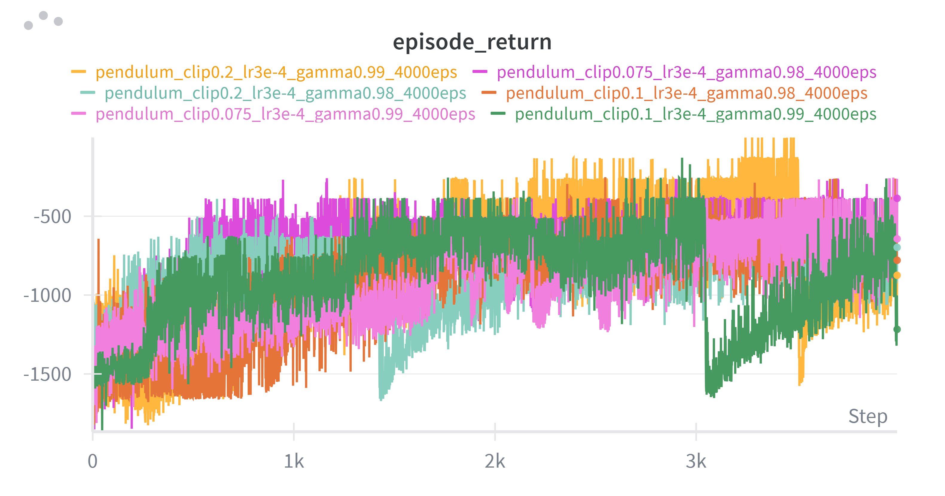
奖励曲线
可视化Pendulum
https://live.csdn.net/v/502372
性能对比 (按超参数分组)
说明: clip=ε (裁剪参数), lr=学习率, gamma=γ (折扣因子), episodes=训练回合数
Gamma = 0.99
| 序号 | Clip (ε) | Learning Rate | Episodes | 平均回报 | 标准差 | 最大值 | 最小值 |
|---|---|---|---|---|---|---|---|
| 1 | 0.075 | 3e-4 | 4000 | -615.28 | 192.78 | -382.76 | -1030.82 |
| 2 | 0.100 | 3e-4 | 4000 | -642.60 | 126.50 | -430.90 | -857.06 |
| 3 | 0.200 | 3e-4 | 4000 | -215.51 | 112.95 | -1.79 | -379.08 |
Gamma = 0.98
| 序号 | Clip (ε) | Learning Rate | Episodes | 平均回报 | 标准差 | 最大值 | 最小值 |
|---|---|---|---|---|---|---|---|
| 4 | 0.075 | 3e-4 | 4000 | -768.82 | 75.34 | -631.76 | -875.19 |
| 5 | 0.100 | 3e-4 | 4000 | -562.52 | 140.26 | -266.61 | -751.72 |
| 6 | 0.200 | 3e-4 | 4000 | -695.30 | 93.90 | -515.69 | -859.87 |
总体性能
| 序号 | Gamma | Clip (ε) | Learning Rate | Episodes | 平均回报 | 标准差 |
|---|---|---|---|---|---|---|
| 1 | 0.99 | 0.200 | 3e-4 | 4000 | -215.51 | 112.95 |
| 2 | 0.98 | 0.100 | 3e-4 | 4000 | -562.52 | 140.26 |
| 3 | 0.99 | 0.075 | 3e-4 | 4000 | -615.28 | 192.78 |
| 4 | 0.99 | 0.100 | 3e-4 | 4000 | -642.60 | 126.50 |
| 5 | 0.98 | 0.200 | 3e-4 | 4000 | -695.30 | 93.90 |
| 6 | 0.98 | 0.075 | 3e-4 | 4000 | -768.82 | 75.34 |
超参数分析
Gamma 对比
- Gamma = 0.99: 平均表现较好,最佳配置为 clip=0.2, 平均回报 -215.51
- Gamma = 0.98: 整体表现较差,最佳配置为 clip=0.1, 平均回报 -562.52
Clip (ε) 对比
Gamma = 0.99 组:
- clip=0.075: 平均回报 -615.28 (较差)
- clip=0.100: 平均回报 -642.60 (最差)
- clip=0.200: 平均回报 -215.51 ⭐ (最优)
Gamma = 0.98 组:
- clip=0.075: 平均回报 -768.82 (最差)
- clip=0.100: 平均回报 -562.52 (较好)
- clip=0.200: 平均回报 -695.30 (较差)
结论
- 最佳超参数组合: Gamma=0.99, Clip=0.2, LR=3e-4
- Gamma影响: 0.99 比 0.98 整体表现更好
- Clip影响 :
- 在 Gamma=0.99 时,较大的 clip (0.2) 效果最好
- 在 Gamma=0.98 时,中等的 clip (0.1) 效果较好
4、调参分析
Clip 参数 (ε) - 裁剪参数
定义
在 PPO-clip 算法中,clip 参数 ε 用于限制策略更新的幅度,防止新策略与旧策略偏离过大。
数学公式
L^CLIP(θ) = E_t[min(r_t(θ)·A_t, clip(r_t(θ), 1-ε, 1+ε)·A_t)]

其中:
- r_t(θ) = π_θ(a_t|s_t) / π_θ_old(a_t|s_t)  # 概率比
- A_t 是优势函数
- clip(x, a, b) 将 x 限制在 [a, b] 范围内
工作机制
当 A_t > 0 (好的动作):
- 如果 r_t > 1+ε: 被裁剪到 1+ε,防止过度鼓励
- 如果 r_t < 1-ε: 不裁剪,允许增加概率
- 目标: 适度增加好动作的概率
当 A_t < 0 (坏的动作):
- 如果 r_t < 1-ε: 被裁剪到 1-ε,防止过度惩罚
- 如果 r_t > 1+ε: 不裁剪,允许减少概率
- 目标: 适度减少坏动作的概率
作用总结
- 训练稳定性: 防止因更新步长过大导致性能崩溃
- 保守更新: 确保新策略不会与旧策略偏离太远
- 避免局部最优: 允许适度探索,避免过早收敛
Gamma 参数 (γ) - 折扣因子
定义
γ 是折扣因子,用于计算未来奖励的现值,控制智能体对短期奖励和长期奖励的权衡。
数学公式
# 累积回报 (Discounted Return)
G_t = r_t + γ·r_{t+1} + γ²·r_{t+2} + ... = Σ(γ^k · r_{t+k})

# TD 目标
y_t = r_t + γ·V(s_{t+1})

# GAE (Generalized Advantage Estimation)
A^GAE(γ,λ)_t = Σ((γλ)^l · δ_{t+l})
其中 δ_t = r_t + γ·V(s_{t+1}) - V(s_t)
工作机制
γ ≈ 1 (如 0.99):
- 重视长期奖励
- 适合需要长期规划的任务
- 学习曲线可能更平滑但收敛较慢
γ ≈ 0 (如 0.5):
- 重视短期奖励
- 适合短期反馈明确的任务
- 学习速度快但可能短视
作用总结
- 时间视野: 控制智能体的"眼界"(看多远的未来)
- 价值估计: 影响状态价值函数 V(s) 的计算
- 学习速度: 影响 TD 误差的传播速度
Gamma 参数影响分析
Gamma = 0.99 组
| Clip | 平均回报 | 性能 | 分析 |
|---|---|---|---|
| 0.075 | -615.28 | 中等 | 过于保守,限制了学习速度 |
| 0.100 | -642.60 | 中等 | 仍然较保守,表现一般 |
| 0.200 | -215.51 | 最优 ⭐ | 适度激进,找到最优策略 |
趋势: Clip 越大,性能越好
Gamma = 0.98 组
| Clip | 平均回报 | 性能 | 分析 |
|---|---|---|---|
| 0.075 | -768.82 | 最差 | 过于保守,严重限制学习 |
| 0.100 | -562.52 | 较好 | 平衡适中,表现相对较好 |
| 0.200 | -695.30 | 较差 | 过于激进,策略不稳定 |
趋势: Clip=0.1 时最优,过小或过大都不好
Gamma 对比
Gamma=0.99 平均表现: (-215.51 + -615.28 + -642.60) / 3 = -491.13
Gamma=0.98 平均表现: (-562.52 + -695.30 + -768.82) / 3 = -675.55

差异: 184.42 (Gamma=0.99 明显更优)
关键发现
1. Gamma=0.99 整体优于 Gamma=0.98
- 原因: Pendulum 是一个需要长期规划的任务
- 倒立摆需要考虑当前动作对未来状态的长期影响
- 更高的 γ 让智能体能"看得更远",做出更好的决策
2. 不同 Gamma 下 Clip 的最优值不同
-
Gamma=0.99: 最优 Clip=0.2 (较大)
- 长期视野下,允许较大的策略更新是有益的
- 能更快地探索和收敛到最优策略
-
Gamma=0.98: 最优 Clip=0.1 (中等)
- 短期视野下,需要更保守的更新
- 过大的 Clip 可能导致短视决策的不稳定
3. 标准差分析
-
最优配置 (0.99, 0.2): 标准差 112.95 (较高)
- 说明策略仍在探索,有些回合表现极好 (-1.79)
- 有较大的改进潜力
-
最差配置 (0.98, 0.075): 标准差 75.34 (较低)
- 策略已经"固化",但固化在较差的局部最优
- 过于保守的更新导致无法逃离
深度解释
为什么 Gamma=0.99 + Clip=0.2 表现最好?
1. Gamma=0.99 的优势
长期规划能力:
python
# 假设 max_steps = 200
# Gamma=0.99: 第 200 步的奖励权重 = 0.99^200 ≈ 0.134
# Gamma=0.98: 第 200 步的奖励权重 = 0.98^200 ≈ 0.018

# 结论: Gamma=0.99 让智能体关注整个回合的表现
#       Gamma=0.98 主要关注前 100 步左右
对 Pendulum 的影响:
- Pendulum 每一步的奖励都是负的:
r = -(θ² + 0.1·θ̇² + 0.001·τ²) - 目标是让倒立摆保持在顶部 (θ=0) 尽可能长的时间
- 需要长期规划: 当前动作 → 影响未来状态 → 影响长期累积奖励
- Gamma=0.99 让智能体学会"牺牲短期,换取长期稳定"
2. Clip=0.2 的优势
适度激进的更新:
python
# Clip=0.2 意味着:
# 概率比 r_t 被限制在 [0.8, 1.2]
# 即新策略与旧策略的概率比最多相差 20%

# 对比:
# Clip=0.075: [0.925, 1.075] - 只允许 7.5% 的变化 (太保守)
# Clip=0.100: [0.900, 1.100] - 允许 10% 的变化 (较保守)
# Clip=0.200: [0.800, 1.200] - 允许 20% 的变化 (适度)
为什么适度激进有效:
- 探索效率: 允许较大的策略变化 → 更快探索状态空间
- 收敛速度: 在找到好策略后,能更快收敛
- 避免局部最优: 有足够的"勇气"跳出局部最优
3. 协同效应
Gamma=0.99 (长期视野) + Clip=0.2 (大步更新)
    ↓
智能体能够:
1. 看到长期收益 (Gamma 高)
2. 快速调整策略去追求长期收益 (Clip 大)
3. 在 4000 回合内找到接近最优的策略
    ↓
最好回合达到 -1.79 (接近理想值 0)
为什么 Gamma=0.98 + Clip=0.2 表现较差?
短视 + 激进 = 不稳定:
Gamma=0.98 (短期视野) + Clip=0.2 (大步更新)
    ↓
问题:
1. 智能体只关注近期奖励 (Gamma 低)
2. 策略变化过快 (Clip 大)
3. 容易被短期噪声误导
    ↓
策略在不同局部最优间震荡
平均回报 -695.30 (较差)
更详细的解释:
- Gamma=0.98 让智能体"短视",只看重前 100 步左右
- Clip=0.2 允许每次大幅调整策略
- 结果: 智能体根据短期反馈大幅调整策略,导致不稳定
- 就像一个只看眼前的人,走路步子还很大,容易摔跤
为什么 Gamma=0.98 + Clip=0.1 相对较好?
短视 + 保守 = 稳定但次优:
Gamma=0.98 (短期视野) + Clip=0.1 (小步更新)
    ↓
特点:
1. 虽然短视,但更新保守
2. 策略变化平稳,避免了震荡
3. 能找到一个"还不错"的局部最优
    ↓
平均回报 -562.52 (次优)
核心洞察
- Gamma 是基础: 先确定正确的 Gamma,它决定了任务的"时间尺度"
- Clip 是调节器: 在正确的 Gamma 下,Clip 控制探索-利用的平衡
- 协同效应: Gamma 和 Clip 需要配合,不能独立优化
- 任务特性优先: 根据任务特点选择参数,而不是固定套路