R语言第七章线性回归模型

R语言第七章线性回归模型

• 7.1数据集
• • 例题：
  • • 方式一：
    • 方式二：
    • tapply函数含义
• 计算喷发时间间隔喷发次数
• • • cumsum()
    • ecdf()函数
    • R绘制茎叶图函数stem()
• 7.2数据的数值度量
• • summary
  • var, sd, cov, cor
• 回归分析
• 根据回归系数lm进行预测
• • 第一种方法
  • 第二种方法
• 多元线性回归分析

如要将代码进行本地运行，建议自上而下运行全文，完整代码放置文末。

7.1数据集

数据集是用于分析和建模的数据集合，通常包含 样本（数据点）、特征（变量）和 标签（目标变量）。

R语言中有很多内置数据集，常见包括 1. iris 2. faithful 3. mtcars

library(help = "datasets")

head(iris)
iris$Species -> SP
(iris.freq <- table(SP))
cbind(iris.freq)
special.relfreq <- iris.freq / nrow(iris);special.relfreq

options函数用于更改保留小数的位数。

#保留任意位小数
old <- options(digits = 2)
special.relfreq
options(old)

barplot(iris.freq)#柱状图查看频次
pie(iris.freq, col = c("red", "green", "yellow"))#饼图查看频次

例题：

求setosa花萼长度的平均值，结果保留3位小数

方式一：

species <- iris$Species
s_species <- species == "setosa"
s_iris <- iris[s_species,]
options(digit = 3) -> old
mean(s_iris$Sepal.Length)

方式二：

tapply函数含义

:第一个参数表示对什么数据进行处理， 第二个参数表示以什么作为划分，第三个参数表示对第一个参数怎么处理。

tapply(iris$Sepal.Length, iris$Species, mean) 

计算喷发时间间隔喷发次数

data(faithful)
head(faithful)
range(faithful$eruptions) #表示泉水喷发的数据范围

#对其faithful$eruptions进行分组
breaks <- seq(1.5, 5.5, by = 0.5) 
cut(faithful$eruptions, breaks, right = F) -> tep #对数据进行分区间操作
freq <- table(tep) #用table函数统计
#或者
hist(faithful$eruptions, right = F)#hist()函数绘制直方图时会自动进行区间（ bins ）划分
#计算相对频数
relfreq <- freq / nrow(faithful)

cumsum()

能够计算向量元素的累加和

cumsum(1:10)
#用cumsum函数计算累计频数分布图
cumsum(freq) -> cumfreq0
plot(breaks,
     c(0, cumfreq0),
     main = "泉水喷发持续时间",
     ylable = "累计喷发频数",
     xlable = "持续时间"
     )
lines(breaks, c(0, cumfreq0))
#添加网格线，不会的看我上一篇
abline(v = seq(0,6,by = 0.5), h = seq(0,300,by = 10), lty = 2, col = "lightgrey")

上一篇

ecdf()函数

用于计算经验累积分布函数（Empirical Cumulative Distribution Function)

ecdf_eruptions <- ecdf(faithful$eruptions) #记住用法即可
plot(ecdf_eruptions,
     main = "泉水喷发持续时间",
     ylable = "累计喷发频数",
     xlable = "持续时间"
     )
#绘制散点图eruption vs waiting
eruption <- faithful$eruptions
waiting <- faithful$waiting
head(cbind(eruption, waiting))
plot(eruption, waiting,
     main = "泉水喷发持续时间与等待时间关系图",
     xlab = "喷发持续时间",
     ylab = "等待时间"
     )

R绘制茎叶图函数stem()

含义：

每个数据点被拆分为：

1. 茎：表示数据的高位部分（如十位数）
2. 叶：表示数据的低位部分（如个位数） 例如：数据点 42 可表示为： 4 2 \begin{array}{c|c} 4 & 2 \ \end{array} 42

stem(faithful$eruptions) #茎叶图

7.2数据的数值度量

求均值函数mean

求中位数函数median

求四分位数函数quantile

求极差函数range

求变化范围max - min

四分位距函数IQR

#求均值函数mean：
mean(faithful$eruptions)
#求中位数函数median：
median(faithful$eruptions)
#求四分位数函数quantile：
quantile(faithful$eruptions)
#求极差函数range：
range(faithful$eruptions)
#求变化范围
max(faithful$eruptions) - min(faithful$eruptions)
#四分位距函数IQR：
IQR(faithful$eruptions)

画出喷发时间和等待时间的箱线图

#画出喷发时间和等待时间的箱线图
par(mfrow = c(1,2))
boxplot(faithful$eruptions)
boxplot(faithful$waiting)
par(mfrow = c(1,1))

summary

函数用于给出数据的五数概括

最小值：数据中的最小观测值

第一四分位数（ Q 1 Q_1 Q1）：数据中25%的观测值小于该值

中位数（ Q 2 Q_2 Q2）：数据排序后正中间的数值

第三四分位数（ Q 3 Q_3 Q3）：数据中75%的观测值小于该值

最大值：数据中的最大观测值

summary(faithful)

var, sd, cov, cor

var（方差）、sd（标准差）、cov（协方差）和 cor（相关系数）

注：相关系数和回归系数是两个不同的统计概念，不要混淆

#求方差var
var(faithful$eruptions)
#求标准差sd
sd(faithful$eruptions)
#求协方差函数cov：
cov(eruption, waiting)
#求相关系数函数cor：
cor(eruption, waiting)

下面的部分的学习建议首先了解概率论与数理统计的基础知识--------------

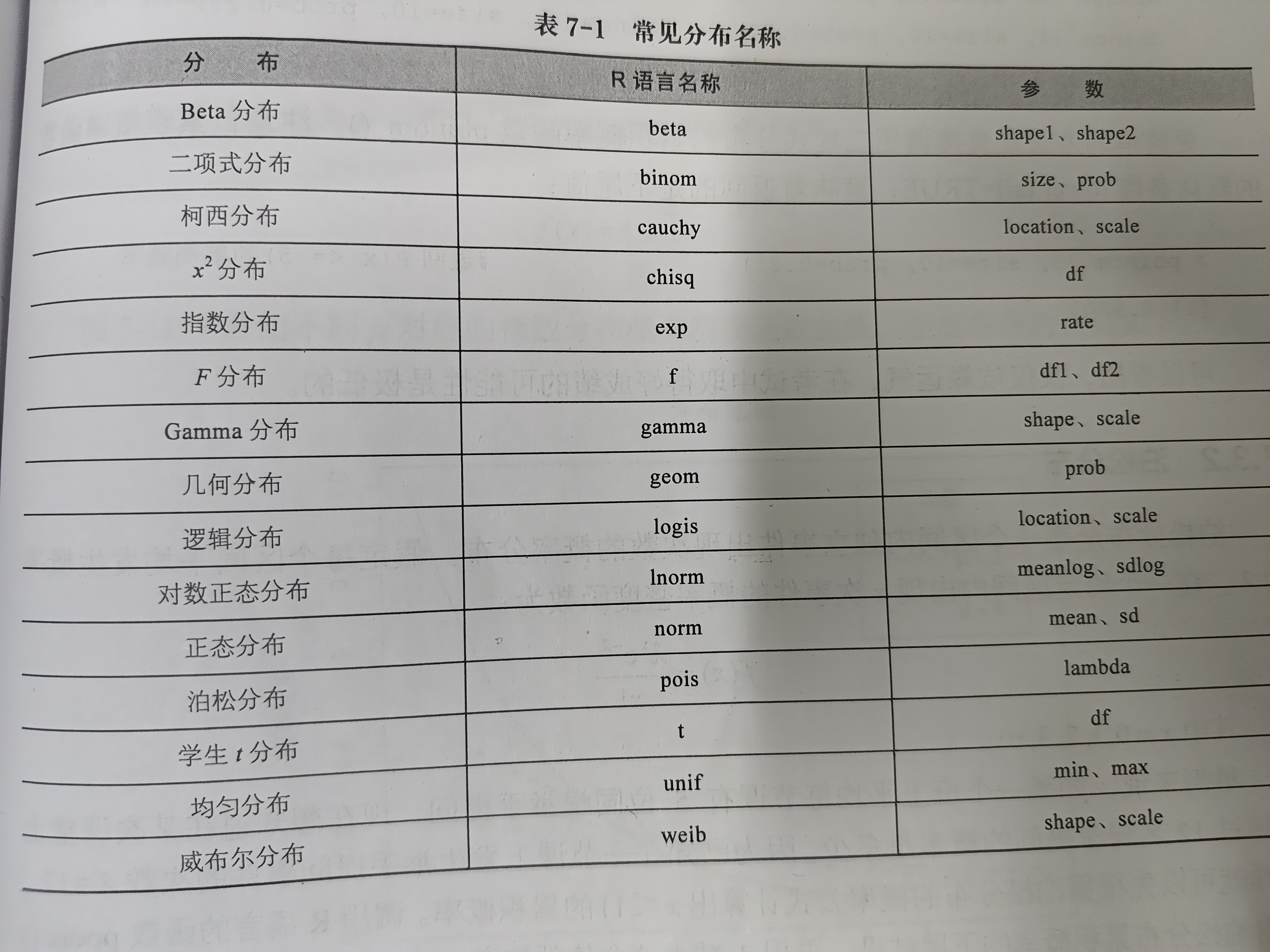
r语言提供了一组函数，分别以d p q r 开头，分别表示不同的含义：

d开头 : 概率密度函数

p开头 : 累积分布函数

q开头 : 分位数函数

r开头 : 随机数生成函数

可以配合许多函数使用，如正态分布norm、t分布t、卡方分布chisq、F分布f等

回归分析

eruption.lm <- lm(eruption ~ waiting, data = faithful);
#显示回归方程中的系数两种方法
1.
coeffs <- eruption.lm $ coefficients
2.
coeffs <- coefficients(eruption.lm);coeffs
#绘制散点图并添加回归直线
plot(eruption ~ waiting, data = faithful,
    col = "blue",
    main = "泉水喷发持续时间与等待时间关系图",
    xlab = "喷发持续时间",
    ylab = "等待时间"
    );
fit <- lm(eruption ~ waiting, data = faithful);
abline(fit, col = "red", lwd = 2);

根据回归系数lm进行预测

第一种方法

#预测喷发时间 
waiting.time <- 80
duration.predict <- coeffs[1] + coeffs[2] * waiting.time
duration.predict

第二种方法

predict函数：参数中需要包含回归系数lm,和一个数据框（要包含除要预测的值外所有的已知参数）且需要确保新数据框的变量名称与模型中使用的变量名称一致

#预测喷发时间 
newdata <- data.frame(waiting = 80)
predict(eruption.lm, newdata)

多元线性回归分析

需要装载r语言数据集BostonHousing（Boston房价）。

install.packages("mlbench")
library(mlbench)
data(BostonHousing)
dim(BostonHousing)
head(BostonHousing)
#了解其数据结构
str(BostonHousing)
boston.lm <- lm(medv ~ ., data = BostonHousing)
boston.lm
#查看回归分析结果
summary(boston.lm)
#预测房价
newdata <- data.frame(crim = 0.03, zn = 90, indus = 2, chas = as.factor(0),
                      nox = 0.5, rm = 7, age = 15, dis = 6,
                      rad = 3, tax = 400, ptratio = 15, b = 400,
                      lstat = 5)
predict(boston.lm, newdata, interval = "predict")#参数interval表示预测区间

整体代码如下:

#首先了解有什么常用的数据集
#常见包括 1. iris 2. faithful 3. mtcars
library(help = "datasets")

head(iris)
iris$Species -> SP
(iris.freq <- table(SP))
cbind(iris.freq)
special.relfreq <- iris.freq / nrow(iris);special.relfreq

#保留任意未小数
old <- options(digits = 2)
special.relfreq
options(old)

barplot(iris.freq)#柱状图查看频次
pie(iris.freq, col = c("red", "green", "yellow"))#饼图查看频次

#例题：求setosa花萼长度的平均值，结果保留3位小数
#方式一：
species <- iris$Species
s_species <- species == "setosa"
s_iris <- iris[s_species,]
options(digit = 3) -> old
mean(s_iris$Sepal.Length)
#方式二：
#tapply函数含义，第一个参数表示对什么数据进行处理， 第二个参数表示以什么作为划分，第三个参数表示对第一个参数怎么处理。
tapply(iris$Sepal.Length, iris$Species, mean) 

data(faithful)
head(faithful)
range(faithful$eruptions) #表示泉水喷发的数据范围

#对其faithful$eruptions进行分组
breaks <- seq(1.5, 5.5, by = 0.5) 
cut(faithful$eruptions, breaks, right = F) -> tep #对数据进行分区间操作
freq <- table(tep) #用table函数统计
#或者
hist(faithful$eruptions, right = F)#hist()函数绘制直方图时会自动进行区间（ bins ）划分
#计算相对频数
relfreq <- freq / nrow(faithful)

#cumsum()能够计算向量元素的累加和
cumsum(1:10)
#用cumsum函数计算累计频数分布图
cumsum(freq) -> cumfreq0
plot(breaks,
     c(0, cumfreq0),
     main = "泉水喷发持续时间",
     ylable = "累计喷发频数",
     xlable = "持续时间"
     )
lines(breaks, c(0, cumfreq0))
#添加网格线，不会的看我上一篇
abline(v = seq(0,6,by = 0.5), h = seq(0,300,by = 10), lty = 2, col = "lightgrey")

#ecdf()函数用于计算经验累积分布函数（Empirical Cumulative Distribution Function)
ecdf_eruptions <- ecdf(faithful$eruptions) #记住用法就行
plot(ecdf_eruptions,
     main = "泉水喷发持续时间",
     ylable = "累计喷发频数",
     xlable = "持续时间"
     )
#绘制散点图eruption vs waiting
eruption <- faithful$eruptions
waiting <- faithful$waiting
head(cbind(eruption, waiting))
plot(eruption, waiting,
     main = "泉水喷发持续时间与等待时间关系图",
     xlab = "喷发持续时间",
     ylab = "等待时间"
     )
#R绘制茎叶图函数stem()
stem(faithful$eruptions) #茎叶图

# 7.2数据的数值度量
#求均值函数mean：
mean(faithful$eruptions)
#求中位数函数median：
median(faithful$eruptions)
#求四分位数函数quantile：
quantile(faithful$eruptions)
#求极差函数range：
range(faithful$eruptions)
#求变化范围
max(faithful$eruptions) - min(faithful$eruptions)
#四分位距函数IQR：
IQR(faithful$eruptions)

#画出喷发时间和等待时间的箱线图
par(mfrow = c(1,2))
boxplot(faithful$eruptions)
boxplot(faithful$waiting)
par(mfrow = c(1,1))

#summary函数用于给出数据的五数概括
summary(faithful)

#求方差函数var和标准差函数sd：
var(faithful$eruptions)
sd(faithful$eruptions)
#求协方差函数cov：
cov(eruption, waiting)
#求相关系数函数cor：
cor(eruption, waiting)


#回归分析
eruption.lm <- lm(eruption ~ waiting, data = faithful);
#显示回归方程中的系数
1.
coeffs <- eruption.lm $ coefficients
2.
coeffs <- coefficients(eruption.lm);coeffs
#绘制散点图并添加回归直线
plot(eruption ~ waiting, data = faithful,
    col = "blue",
    main = "泉水喷发持续时间与等待时间关系图",
    xlab = "喷发持续时间",
    ylab = "等待时间"
    );
fit <- lm(eruption ~ waiting, data = faithful);
abline(fit, col = "red", lwd = 2);
#预测喷发时间 第一种方法
waiting.time <- 80
duration.predict <- coeffs[1] + coeffs[2] * waiting.time
duration.predict
#预测喷发时间 第二种方法
newdata <- data.frame(waiting = 80)
predict(eruption.lm, newdata)

#多元线性回归分析
install.packages("mlbench")
library(mlbench)
data(BostonHousing)
dim(BostonHousing)
head(BostonHousing)
#了解其数据结构
str(BostonHousing)
boston.lm <- lm(medv ~ ., data = BostonHousing)
boston.lm
#查看回归分析结果
summary(boston.lm)
#预测房价
newdata <- data.frame(crim = 0.03, zn = 90, indus = 2, chas = as.factor(0),
                      nox = 0.5, rm = 7, age = 15, dis = 6,
                      rad = 3, tax = 400, ptratio = 15, b = 400,
                      lstat = 5)
predict(boston.lm, newdata, interval = "predict")#参数interval表示预测区间```