深度学习实战（基于pytroch）系列（三十八）门控循环单元（GRU）从零开始实现

门控循环单元（GRU）从零开始实现

门控循环单元

前面我们讨论了循环神经网络中的梯度计算方法。我们发现，当时间步数较大或较小时，循环神经网络的梯度容易发生衰减或爆炸。虽然梯度裁剪可以处理梯度爆炸问题，但无法解决梯度衰减的挑战。正因如此，循环神经网络在实际应用中往往难以有效捕捉时间序列中跨度较大的依赖关系。

门控循环神经网络（gated recurrent neural network）的设计初衷，就是为了更好地建模时间序列中长期依赖关系。它通过可学习的门控机制来调节信息流动。其中，门控循环单元（gated recurrent unit，GRU）是一种广泛使用的门控循环神经网络。

门控循环单元原理

下面详细介绍门控循环单元的设计思想。它引入了重置门（reset gate）和更新门（update gate）的概念，对传统循环神经网络的隐藏状态计算方式进行了改进。

重置门和更新门

如图所示，门控循环单元中的重置门和更新门的输入都是当前时间步输入 X t X_t Xt与上一时间步隐藏状态 H t − 1 H_{t-1} Ht−1，输出由sigmoid激活函数的全连接层计算得到。

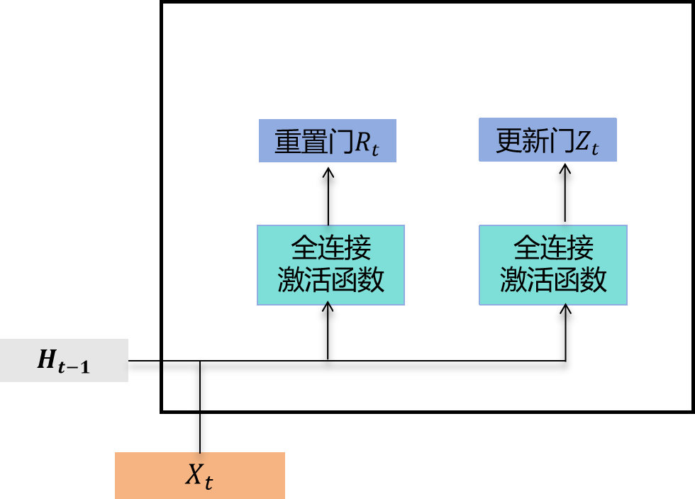
具体而言，假设隐藏单元个数为 h h h，给定时间步 t t t的小批量输入 X t ∈ R n × d X_t \in \mathbb{R}^{n \times d} Xt∈Rn×d（样本数为 n n n，输入维度为 d d d）和上一时间步隐藏状态 H t − 1 ∈ R n × h H_{t-1} \in \mathbb{R}^{n \times h} Ht−1∈Rn×h。重置门 R t ∈ R n × h R_t \in \mathbb{R}^{n \times h} Rt∈Rn×h和更新门 Z t ∈ R n × h Z_t \in \mathbb{R}^{n \times h} Zt∈Rn×h的计算公式为：

R t = σ ( X t W x r + H t − 1 W h r + b r ) R_t = \sigma(X_t W_{xr} + H_{t-1} W_{hr} + b_r) Rt=σ(XtWxr+Ht−1Whr+br)
Z t = σ ( X t W x z + H t − 1 W h z + b z ) Z_t = \sigma(X_t W_{xz} + H_{t-1} W_{hz} + b_z) Zt=σ(XtWxz+Ht−1Whz+bz)

其中 W x r , W x z ∈ R d × h W_{xr}, W_{xz} \in \mathbb{R}^{d \times h} Wxr,Wxz∈Rd×h和 W h r , W h z ∈ R h × h W_{hr}, W_{hz} \in \mathbb{R}^{h \times h} Whr,Whz∈Rh×h是权重参数， b r , b z ∈ R 1 × h b_r, b_z \in \mathbb{R}^{1 \times h} br,bz∈R1×h是偏置参数。如"多层感知机"一节所述，sigmoid函数能将元素值压缩到0和1之间。因此，重置门 R t R_t Rt和更新门 Z t Z_t Zt中每个元素的取值范围都是 [ 0 , 1 ] [0, 1] [0,1]。

候选隐藏状态

接下来，门控循环单元会计算候选隐藏状态以辅助后续的隐藏状态计算。如下图所示，我们将当前时间步重置门的输出与上一时间步隐藏状态进行逐元素乘法（符号为 ⊙ \odot ⊙）。如果重置门中某个元素值接近0，意味着对应隐藏状态元素将被重置为0，即丢弃上一时间步的隐藏信息。如果元素值接近1，则表示保留上一时间步的隐藏状态。然后，将逐元素乘法的结果与当前时间步的输入拼接，再通过包含tanh激活函数的全连接层计算候选隐藏状态，其所有元素的值域为 [ − 1 , 1 ] [-1, 1] [−1,1]（tanh函数的范围）。

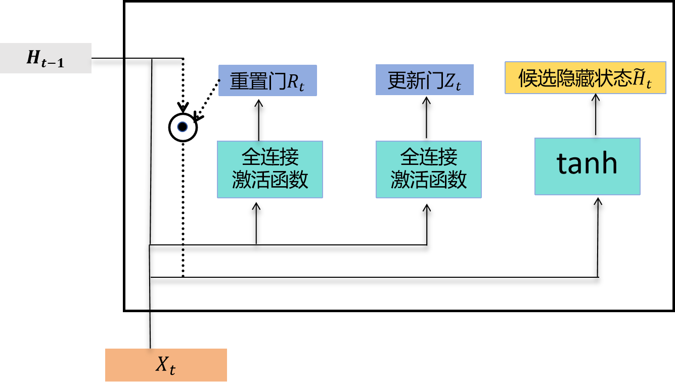
门控循环单元中候选隐藏状态的计算。这里的 ⊙ \odot ⊙表示逐元素乘法

具体来说，时间步 t t t的候选隐藏状态 H ~ t ∈ R n × h \tilde{H}_t \in \mathbb{R}^{n \times h} H~t∈Rn×h的计算公式为：

H ~ t = tanh ⁡ ( X t W x h + ( R t ⊙ H t − 1 ) W h h + b h ) \tilde{H}t = \tanh(X_t W{xh} + (R_t \odot H_{t-1}) W_{hh} + b_h) H~t=tanh(XtWxh+(Rt⊙Ht−1)Whh+bh)

其中 W x h ∈ R d × h W_{xh} \in \mathbb{R}^{d \times h} Wxh∈Rd×h和 W h h ∈ R h × h W_{hh} \in \mathbb{R}^{h \times h} Whh∈Rh×h是权重参数， b h ∈ R 1 × h b_h \in \mathbb{R}^{1 \times h} bh∈R1×h是偏置参数。从这个公式可以看出，重置门控制了上一时间步的隐藏状态如何影响当前时间步的候选隐藏状态。由于上一时间步的隐藏状态可能包含了截至该时间步的全部历史信息，因此重置门可用于丢弃与当前预测无关的历史信息。

隐藏状态

最后，时间步 t t t的隐藏状态 H t ∈ R n × h H_t \in \mathbb{R}^{n \times h} Ht∈Rn×h的计算使用当前时间步的更新门 Z t Z_t Zt来组合上一时间步的隐藏状态 H t − 1 H_{t-1} Ht−1和当前时间步的候选隐藏状态 H ~ t \tilde{H}_t H~t：

H t = Z t ⊙ H t − 1 + ( 1 − Z t ) ⊙ H ~ t H_t = Z_t \odot H_{t-1} + (1 - Z_t) \odot \tilde{H}_t Ht=Zt⊙Ht−1+(1−Zt)⊙H~t

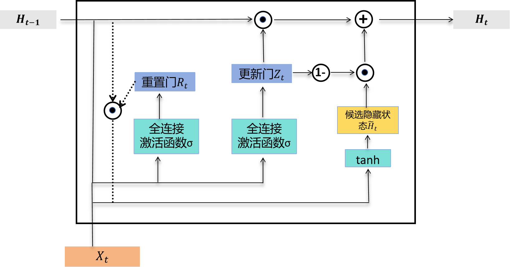
门控循环单元中隐藏状态的计算。这里的 ⊙ \odot ⊙表示逐元素乘法

值得注意的是，更新门可以控制隐藏状态应该如何被包含当前时间步信息的候选隐藏状态所更新，如图所示。假设更新门在时间步 t ′ t' t′到 t t t（ t ′ < t t' < t t′<t）之间始终保持接近1的值。那么，在时间步 t ′ t' t′到 t t t之间的输入信息几乎不会影响时间步 t t t的隐藏状态 H t H_t Ht。实际上，这可以视为较早时刻的隐藏状态 H t ′ − 1 H_{t'-1} Ht′−1直接传递到当前时间步 t t t。这种设计能够缓解循环神经网络中的梯度衰减问题，并更好地捕捉时间序列中跨度较大的依赖关系。

我们对门控循环单元的设计做一个简要总结：

重置门有助于捕捉时间序列中的短期依赖关系；
更新门有助于捕捉时间序列中的长期依赖关系。

读取数据集

为了实现和演示门控循环单元，我们继续使用周杰伦歌词数据集来训练模型进行歌词创作。这里除门控循环单元以外的实现已在"循环神经网络"一节中介绍过。以下是读取数据集部分。

python 复制代码

import torch
import torch.nn as nn
import torch.optim as optim
import math
import random
import time
import zipfile

def load_data_jay_lyrics():
    with zipfile.ZipFile('../data/jaychou_lyrics.txt.zip') as zin:
        with zin.open('jaychou_lyrics.txt') as f:
            corpus_chars = f.read().decode('utf-8')
    corpus_chars = corpus_chars.replace('\n', ' ').replace('\r', ' ')
    corpus_chars = corpus_chars[0:10000]
    idx_to_char = list(set(corpus_chars))
    char_to_idx = {char: i for i, char in enumerate(idx_to_char)}
    vocab_size = len(char_to_idx)
    corpus_indices = [char_to_idx[char] for char in corpus_chars]
    return corpus_indices, char_to_idx, idx_to_char, vocab_size


(corpus_indices, char_to_idx, idx_to_char, vocab_size) = load_data_jay_lyrics()

从零开始实现

我们首先介绍如何从零开始实现门控循环单元。

初始化模型参数

下面的代码对模型参数进行初始化。超参数num_hiddens定义了隐藏单元的数量。本质上这里和之前"循环神经网络"中的参数初始化差不多，只是多了重置门和更新门所对应的参数初始化。

python 复制代码

num_inputs, num_hiddens, num_outputs = vocab_size, 256, vocab_size
ctx = d2l.try_gpu()

def get_params():
    def _one(shape):
        return nn.Parameter(torch.randn(shape, device=ctx) * 0.01)
    
    def _three():
        return (_one((num_inputs, num_hiddens)),
                _one((num_hiddens, num_hiddens)),
                nn.Parameter(torch.zeros(num_hiddens, device=ctx)))
    
    # 更新门参数
    W_xz, W_hz, b_z = _three()
    # 重置门参数
    W_xr, W_hr, b_r = _three()
    # 候选隐藏状态参数
    W_xh, W_hh, b_h = _three()
    # 输出层参数
    W_hq = _one((num_hiddens, num_outputs))
    b_q = nn.Parameter(torch.zeros(num_outputs, device=ctx))
    
    params = [W_xz, W_hz, b_z, W_xr, W_hr, b_r, W_xh, W_hh, b_h, W_hq, b_q]
    return params

定义模型

下面的代码定义隐藏状态初始化函数init_gru_state。与"循环神经网络的从零开始实现"一节中定义的init_rnn_state函数类似，它返回一个形状为(批量大小, 隐藏单元个数)且初始值为0的张量组成的元组。

python 复制代码

def init_gru_state(batch_size, num_hiddens, device):
    return (torch.zeros((batch_size, num_hiddens), device=device), )

下面根据门控循环单元的计算表达式定义模型。

python 复制代码

def gru(inputs, state, params):
    W_xz, W_hz, b_z, W_xr, W_hr, b_r, W_xh, W_hh, b_h, W_hq, b_q = params
    H, = state
    outputs = []
    
    for X in inputs:
        # 更新门计算
        Z = torch.sigmoid(torch.matmul(X, W_xz) + torch.matmul(H, W_hz) + b_z)
        # 重置门计算
        R = torch.sigmoid(torch.matmul(X, W_xr) + torch.matmul(H, W_hr) + b_r)
        # 候选隐藏状态计算
        H_tilda = torch.tanh(torch.matmul(X, W_xh) + torch.matmul(R * H, W_hh) + b_h)
        # 隐藏状态更新
        H = Z * H + (1 - Z) * H_tilda
        # 输出计算
        Y = torch.matmul(H, W_hq) + b_q
        outputs.append(Y)
    
    return outputs, (H,)

训练模型并创作歌词

我们在训练模型时使用相邻采样。设置好超参数后，我们将训练模型并根据前缀"分开"和"不分开"分别创作长度为50个字符的一段歌词。

python 复制代码

num_epochs, num_steps, batch_size, lr, clipping_theta = 160, 35, 32, 1e2, 1e-2
pred_period, pred_len, prefixes = 40, 50, ['分开', '不分开']

我们每过40个迭代周期便根据当前训练的模型创作一段歌词。这段代码虽然很长，但是里面的方法one_hot，to_onehot,grad_clipping,data_iter_random,data_iter_consecutive,predict_rnn及train_and_predict_rnn均和之前"循环神经网络"中的方法保持一致，最大的区别是模型换成了gru而不是rnn。

python 复制代码

def one_hot(x, n_class, dtype=torch.float32):
    # x shape: (batch_size,), 输出形状: (batch_size, n_class)
    x = x.long()
    res = torch.zeros(x.shape[0], n_class, dtype=dtype, device=x.device)
    res.scatter_(1, x.view(-1, 1), 1)
    return res


def to_onehot(X, n_class):
    # X shape: (batch_size, seq_len), 输出: seq_len个(batch_size, n_class)的Tensor
    return [one_hot(X[:, i], n_class) for i in range(X.shape[1])]


def grad_clipping(params, theta, device):
    norm = torch.tensor([0.0], device=device)
    for param in params:
        norm += (param.grad.data ** 2).sum()
    norm = norm.sqrt().item()
    if norm > theta:
        for param in params:
            param.grad.data *= (theta / norm)


def data_iter_random(corpus_indices, batch_size, num_steps, device=None):
    # 减1是因为输出的索引是相应输入的索引加1
    num_examples = (len(corpus_indices) - 1) // num_steps
    epoch_size = num_examples // batch_size
    example_indices = list(range(num_examples))
    random.shuffle(example_indices)
    
    # 返回从pos开始的长为num_steps的序列
    def _data(pos):
        return corpus_indices[pos: pos + num_steps]
    
    for i in range(epoch_size):
        # 每次读取batch_size个随机样本
        i = i * batch_size
        batch_indices = example_indices[i: i + batch_size]
        X = [_data(j * num_steps) for j in batch_indices]
        Y = [_data(j * num_steps + 1) for j in batch_indices]
        yield torch.tensor(X, device=device), torch.tensor(Y, device=device)

def data_iter_consecutive(corpus_indices, batch_size, num_steps, device=None):
    corpus_indices = torch.tensor(corpus_indices, device=device)
    data_len = len(corpus_indices)
    batch_len = data_len // batch_size
    indices = corpus_indices[0: batch_size * batch_len].reshape(
        batch_size, batch_len)
    epoch_size = (batch_len - 1) // num_steps
    for i in range(epoch_size):
        i = i * num_steps
        X = indices[:, i: i + num_steps]
        Y = indices[:, i + 1: i + num_steps + 1]
        yield X, Y

        
def predict_rnn(prefix, num_chars, rnn, params, init_rnn_state,
                num_hiddens, vocab_size, device, idx_to_char, char_to_idx):
    state = init_rnn_state(1, num_hiddens, device)
    output = [char_to_idx[prefix[0]]]
    for t in range(num_chars + len(prefix) - 1):
        # 将上一时间步的输出作为当前时间步的输入
        X = to_onehot(torch.tensor([[output[-1]]], device=device), vocab_size)
        # 计算输出和更新隐藏状态
        (Y, state) = rnn(X, state, params)
        # 下一个时间步的输入是prefix里的字符或者当前的最佳预测字符
        if t < len(prefix) - 1:
            output.append(char_to_idx[prefix[t + 1]])
        else:
            output.append(int(Y[0].argmax(dim=1).item()))
    return ''.join([idx_to_char[i] for i in output])


def train_and_predict_rnn(rnn, get_params, init_rnn_state, num_hiddens,
                          vocab_size, device, corpus_indices, idx_to_char,
                          char_to_idx, is_random_iter, num_epochs, num_steps,
                          lr, clipping_theta, batch_size, pred_period,
                          pred_len, prefixes):
    if is_random_iter:
        data_iter_fn = data_iter_random
    else:
        data_iter_fn = data_iter_consecutive
    params = get_params()
    loss = nn.CrossEntropyLoss()
    optimizer = optim.SGD(params, lr=lr)
    
    for epoch in range(num_epochs):
        if not is_random_iter:  # 如使用相邻采样，在epoch开始时初始化隐藏状态
            state = init_rnn_state(batch_size, num_hiddens, device)
        l_sum, n, start = 0.0, 0, time.time()
        data_iter = data_iter_fn(corpus_indices, batch_size, num_steps, device)
        for X, Y in data_iter:
            if is_random_iter:  # 如使用随机采样，在每个小批量更新前初始化隐藏状态
                state = init_rnn_state(batch_size, num_hiddens, device)
            else:  # 否则需要使用detach函数从计算图分离隐藏状态
                if isinstance(state, (tuple, list)):
                    for s in state:
                        s.detach_()
                else:
                    state.detach_()
            
            inputs = to_onehot(X, vocab_size)
            # outputs有num_steps个形状为(batch_size, vocab_size)的矩阵
            (outputs, state) = rnn(inputs, state, params)
            # 拼接之后形状为(num_steps * batch_size, vocab_size)
            outputs = torch.cat(outputs, dim=0)
            # Y的形状是(batch_size, num_steps)，转置后再变成长度为
            # batch * num_steps 的向量，这样跟输出的行一一对应
            y = Y.T.reshape(-1)
            
            # 使用交叉熵损失计算平均分类误差
            l = loss(outputs, y.long())
            
            optimizer.zero_grad()
            l.backward()
            grad_clipping(params, clipping_theta, device)  # 裁剪梯度
            optimizer.step()  # 因为误差已经取过均值，梯度不用再做平均
            l_sum += l.item() * y.numel()
            n += y.numel()
        
        if (epoch + 1) % pred_period == 0:
            print('epoch %d, perplexity %f, time %.2f sec' % (
                epoch + 1, math.exp(l_sum / n), time.time() - start))
            for prefix in prefixes:
                print(' -', predict_rnn(
                    prefix, pred_len, rnn, params, init_rnn_state,
                    num_hiddens, vocab_size, device, idx_to_char, char_to_idx))

train_and_predict_rnn(gru, get_params, init_gru_state, num_hiddens,
                          vocab_size, ctx, corpus_indices, idx_to_char,
                          char_to_idx, False, num_epochs, num_steps, lr,
                          clipping_theta, batch_size, pred_period, pred_len,
                          prefixes)

输出示例：

epoch 40, perplexity 152.945260, time 0.09 sec

分开我想你的让我想想想想你想你想你想你想你想你想你想你想你想你想你想你想你想你想你想你想你想你想你想你

不分开我想你的让我想想想想你想你想你想你想你想你想你想你想你想你想你想你想你想你想你想你想你想你想你想你

epoch 80, perplexity 33.027476, time 0.09 sec

分开我想要这样我不要再想我不要再想我不要再想我不要再想我不要再想我不要再想我不要再想我

不分开我想要这样我不要再想我不要再想我不要再想我不要再想我不要再想我不要再想我不要再想我

epoch 120, perplexity 5.928247, time 0.09 sec

分开我想就这样牵着你的手不放开爱可不可以简单单单没有伤害你靠着我的肩膀你在我胸口睡著像这样

不分开我不知不觉我跟了这节奏后知后觉又过了一切秋后知后觉我该好好生活我该好好生活我该好好生

epoch 160, perplexity 1.760153, time 0.09 sec

分开我想就这样牵着你的手不想开说只是我怕眼泪撑不住不懂你的黑色幽默想通却又再考倒我说散你

不分开没有你烦我有多烦恼多难熬穿过云层我试著努力向你奔跑爱才送到你却已在别人怀抱就是开不了

小结

门控循环神经网络能够更好地捕捉时间序列中跨度较大的依赖关系。
门控循环单元引入了门控机制，改进了循环神经网络中隐藏状态的计算方式。它包括重置门、更新门、候选隐藏状态和隐藏状态。
重置门有助于捕捉时间序列中的短期依赖关系。
更新门有助于捕捉时间序列中的长期依赖关系。

本系列目录链接