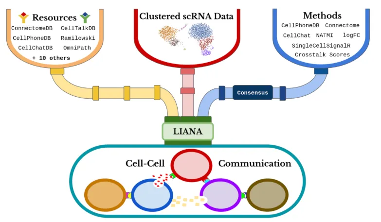
单细胞RNA测序的快速发展激发了人们对细胞间通讯机制的研究兴趣。近年来,已有多种用于研究细胞---细胞通讯(CCC)的工具和数据库被相继开发。然而,这些方法通常是固定绑定的------每种分析工具往往只能与特定的资源配套使用------尽管从原理上讲,任何计算方法都可以与任意配体--受体数据库组合使用。为了解决这一限制,研究团队开发了liana框架,旨在将分析方法与资源解耦,从而实现灵活组合与扩展。
分析流程
1.导入
rm(list=ls())
library(tidyverse)
library(magrittr)
library(SeuratData)
library(liana)
2.数据来源和方法
# CCC资源
# Resource currently included in OmniPathR (and hence `liana`) include:
show_resources()
#  [1] "Default"          "Consensus"        "Baccin2019"       "CellCall"
#  [5] "CellChatDB"       "Cellinker"        "CellPhoneDB"      "CellTalkDB"
#  [9] "connectomeDB2020" "EMBRACE"          "Guide2Pharma"     "HPMR"
# [13] "ICELLNET"         "iTALK"            "Kirouac2010"      "LRdb"
# [17] "Ramilowski2015"   "OmniPath"         "MouseConsensus"

# CCC方法
# Resource currently included in OmniPathR (and hence `liana`) include:
show_methods()
  # [1] "connectome"      "logfc"           "natmi"           "sca"
  # [5] "cellphonedb"     "cytotalk"        "call_squidpy"    "call_cellchat"
  # [9] "call_connectome" "call_sca"        "call_italk"      "call_natmi"
3.准备数据
liana_path <- system.file(package = "liana")
testdata <-
  readRDS(file.path(liana_path , "testdata", "input", "testdata.rds"))

testdata %>% dplyr::glimpse()
# ormal class 'Seurat' [package "SeuratObject"] with 13 slots
#   ..@ assays      :List of 1
#   .. ..$ RNA:Formal class 'Assay' [package "Seurat"] with 8 slots
#   ..@ meta.data   :'data.frame': 90 obs. of  4 variables:
#   .. ..$ orig.ident        : Factor w/ 1 level "pbmc3k": 1 1 1 1 1 1 1 1 1 1 ...
#   .. ..$ nCount_RNA        : num [1:90] 4903 3914 4973 3281 2641 ...
#   .. ..$ nFeature_RNA      : int [1:90] 1352 1112 1445 1015 928 937 899 1713 960 888 ...
#   .. ..$ seurat_annotations: Factor w/ 3 levels "B","CD8 T","NK": 1 1 1 1 3 3 1 1 1 1 ...
#   ..@ active.assay: chr "RNA"
#   ..@ active.ident: Factor w/ 3 levels "B","CD8 T","NK": 1 1 1 1 3 3 1 1 1 1 ...
#   .. ..- attr(*, "names")= chr [1:90] "AAACATTGAGCTAC" "AAACTTGAAAAACG" "AAAGGCCTGTCTAG" "AAAGTTTGGGGTGA" ...
#   ..@ graphs      : list()
#   ..@ neighbors   : list()
#   ..@ reductions  : list()
#   ..@ images      : list()
#   ..@ project.name: chr "SeuratProject"
#   ..@ misc        : list()
#   ..@ version     :Classes 'package_version', 'numeric_version'  hidden list of 1
#   .. ..$ : int [1:3] 3 2 3
#   ..@ commands    :List of 2
#   .. ..$ FindVariableFeatures.RNA:Formal class 'SeuratCommand' [package "Seurat"] with 5 slots
#   .. ..$ NormalizeData.RNA       :Formal class 'SeuratCommand' [package "SeuratObject"] with 5 slots
#   ..@ tools       : list()
4.运行liana
liana_test <- liana_wrap(testdata)

# Liana 会返回一个结果列表,其中的每个元素都对应一种分析方法。
liana_test %>% dplyr::glimpse()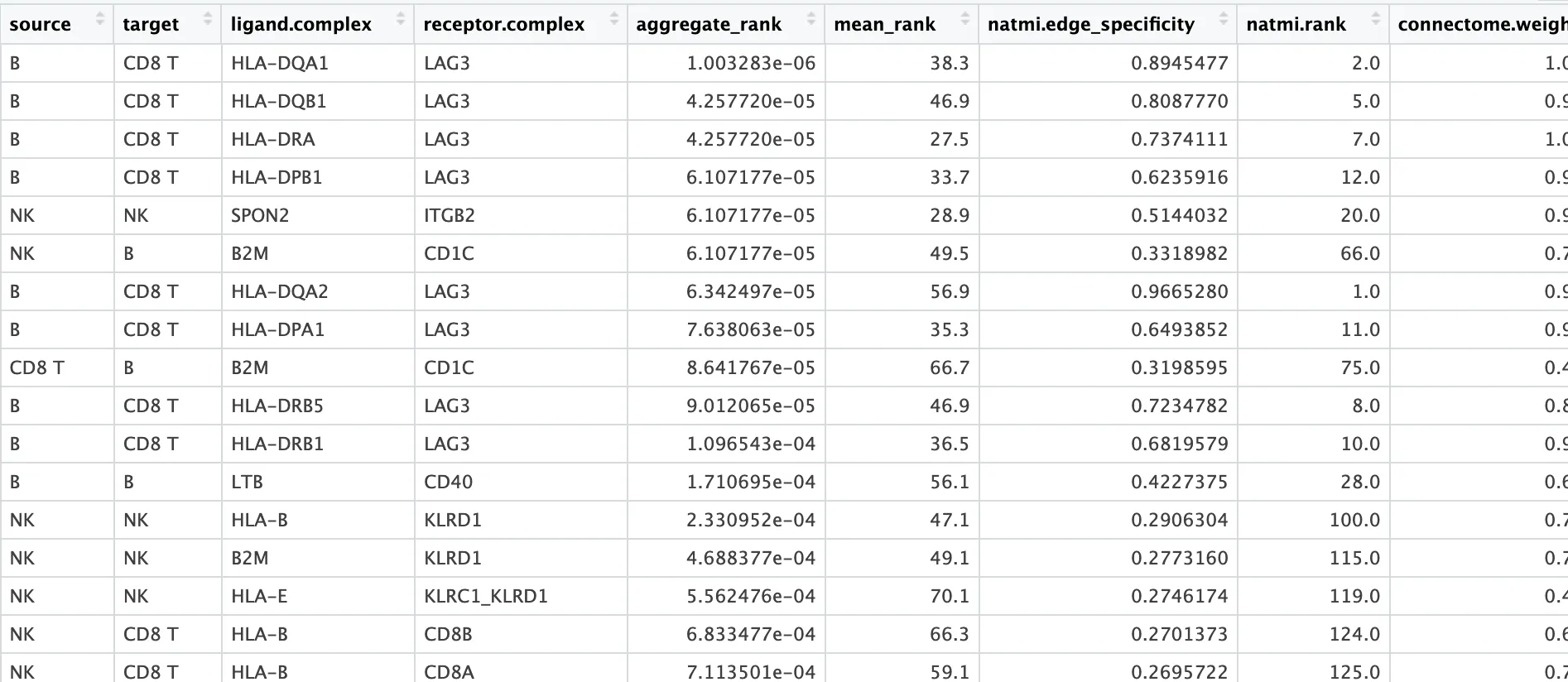
5.聚合并获取共识排序
# 将这些结果聚合为一个包含共识排序的tibble表
liana_test <- liana_test %>%
  liana_aggregate()

dplyr::glimpse(liana_test)
# Rows: 735
# Columns: 16
# $ source                 <chr> "B", "B", "B", "B", "NK", "NK", "B", "B", "CD8 T", "B", "B", "B", ...
# $ target                 <chr> "CD8 T", "CD8 T", "CD8 T", "CD8 T", "NK", "B", "CD8 T", "CD8 T", "...
# $ ligand.complex         <chr> "HLA-DQA1", "HLA-DQB1", "HLA-DRA", "HLA-DPB1", "SPON2", "B2M", "HL...
# $ receptor.complex       <chr> "LAG3", "LAG3", "LAG3", "LAG3", "ITGB2", "CD1C", "LAG3", "LAG3", "...
# $ aggregate_rank         <dbl> 1.003283e-06, 4.257720e-05, 4.257720e-05, 6.107177e-05, 6.107177e-...
# $ mean_rank              <dbl> 38.3, 46.9, 27.5, 33.7, 28.9, 49.5, 56.9, 35.3, 66.7, 46.9, 36.5, ...
# $ natmi.edge_specificity <dbl> 0.8945477, 0.8087770, 0.7374111, 0.6235916, 0.5144032, 0.3318982, ...
# $ natmi.rank             <dbl> 2, 5, 7, 12, 20, 66, 1, 11, 75, 8, 10, 28, 100, 115, 119, 124, 125...
# $ connectome.weight_sc   <dbl> 1.0054344, 0.9026001, 1.0097786, 0.9181296, 0.9000847, 0.7056198, ...
# $ connectome.rank        <dbl> 2, 7, 1, 5, 8, 19, 6, 4, 64, 9, 3, 21, 13, 14, 52, 24, 18, 20, 16,...
# $ logfc.logfc_comb       <dbl> 2.4495727, 2.2335507, 2.7106868, 2.1918963, 2.2886801, 1.0668249, ...
# $ logfc.rank             <dbl> 2, 4, 1, 6, 3, 52, 8, 5, 82, 9, 7, 61, 23, 25, 44, 57, 48, 51, 43,...
# $ sca.LRscore            <dbl> 0.8693937, 0.8561886, 0.8985606, 0.8892920, 0.9046142, 0.9062742, ...
# $ sca.rank               <dbl> 109, 142, 52, 69, 37, 34, 193, 80, 36, 132, 86, 94, 23, 15, 59, 50...
# $ cellphonedb.pvalue     <dbl> 0, 0, 0, 0, 0, 0, 0, 0, 0, 0, 0, 0, 0, 0, 0, 0, 0, 0, 0, 0, 0, 0, ...
# $ cellphonedb.rank       <dbl> 76.5, 76.5, 76.5, 76.5, 76.5, 76.5, 76.5, 76.5, 76.5, 76.5, 76.5, ...
6.简单绘图可视化
6.1. 气泡图
liana_test %>%
  liana_dotplot(source_groups = c("B"),
                target_groups = c("NK", "CD8 T", "B"),
                ntop = 20)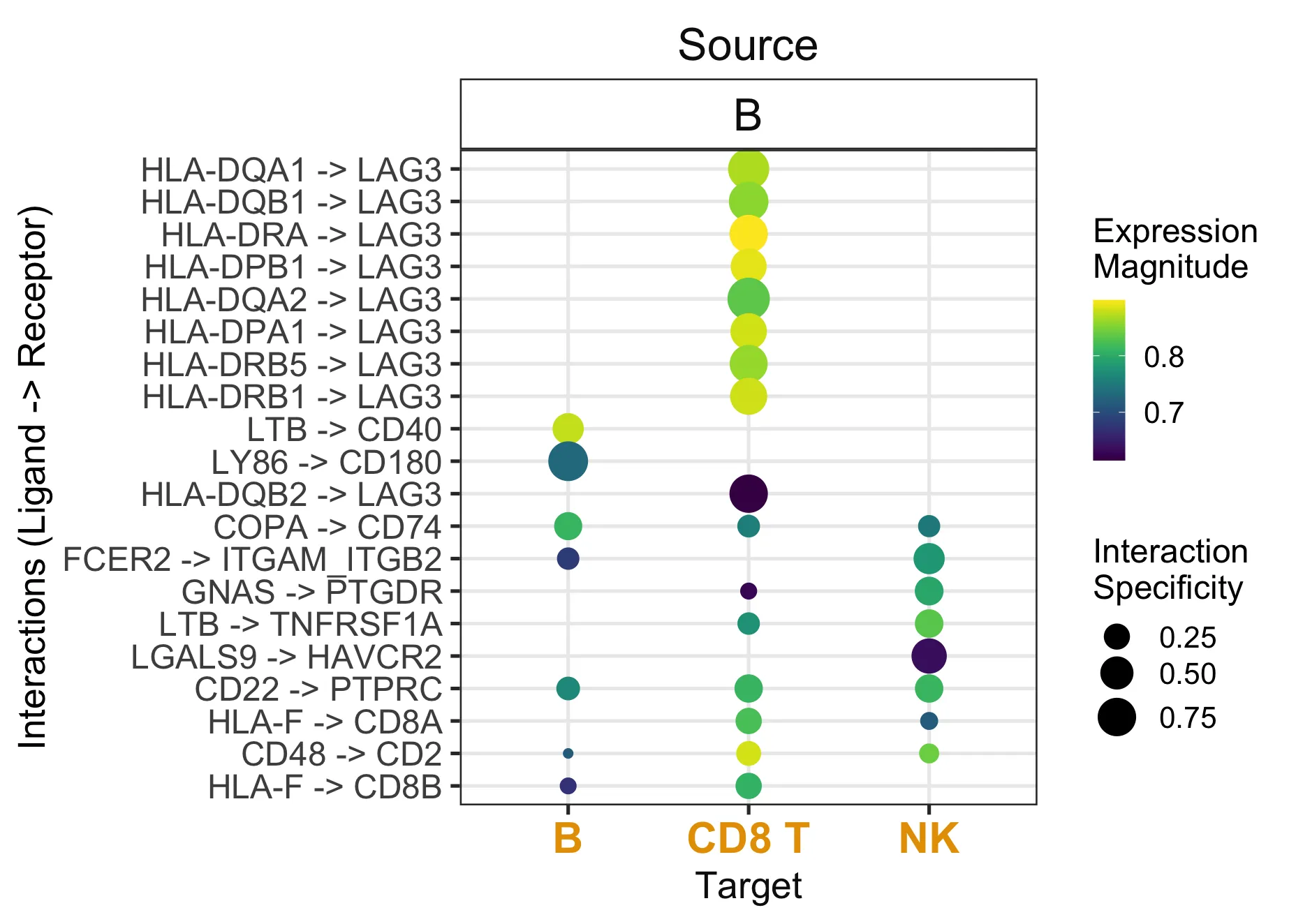
6.2. 频率热图
liana_trunc <- liana_test %>%
   # 仅保留在不同方法之间结果一致的相互作用。
  filter(aggregate_rank <= 0.01)

heat_freq(liana_trunc)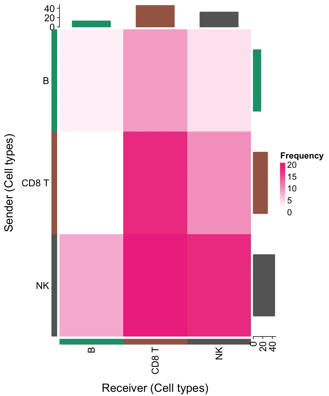
6.3. 频率弦图
# if(!require("circlize")){
#   install.packages("circlize", quiet = TRUE,
#                    repos = "http://cran.us.r-project.org")

p <- chord_freq(liana_trunc,
                source_groups = c("CD8 T", "NK", "B"),
                target_groups = c("CD8 T", "NK", "B"))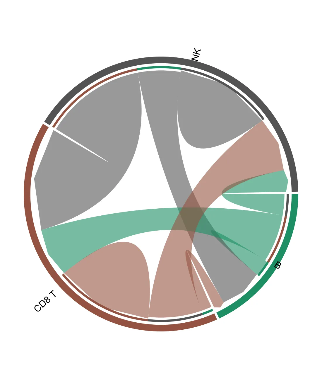
7.选择特定的分析方法
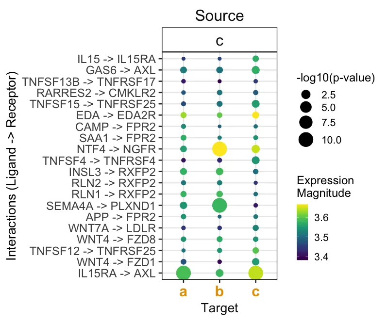
现在只运行 CellPhoneDB的基于置换的算法。同时,为了节省计算时间,会减少置换次数。需要注意的是,LIANA 中实现的 CPDB算法也可以并行化运行。
sce <- readRDS(file.path(liana_path , "testdata", "input", "testsce.rds"))

# RUN CPDB alone
cpdb_test <- liana_wrap(sce,
                        method = 'cellphonedb',
                        resource = c('CellPhoneDB'),
                        permutation.params = list(nperms=100,
                                                  parallelize=FALSE,
                                                  workers=4),
                        expr_prop=0.05)

# 识别感兴趣的相互作用
cpdb_int <- cpdb_test %>%
  # 仅保留 p 值 ≤ 0.1 的相互作用
  filter(pvalue <= 0.1) %>% # 反映了相互作用的"特异性"
  # 根据"强度"(在此例中为 lr_mean)进行排序
  rank_method(method_name = "cellphonedb",
              mode = "magnitude") %>%
  # 保留前 20 个相互作用(不区分细胞类型)
  distinct_at(c("ligand.complex", "receptor.complex")) %>%
  head(20)

# 结果可视化
cpdb_test %>%
  # 仅保留感兴趣的相互作用
  inner_join(cpdb_int,
             by = c("ligand.complex", "receptor.complex")) %>%
  # 反转点的大小(p 值低 / 特异性高 = 点更大)
  # + 对0值添加一个小数值以避免出现无穷大
  mutate(pvalue = -log10(pvalue + 1e-10)) %>%
  liana_dotplot(source_groups = c("c"),
                target_groups = c("c", "a", "b"),
                specificity = "pvalue",
                magnitude = "lr.mean",
                show_complex = TRUE,
                size.label = "-log10(p-value)")