扩散模型简介：The Annotated Diffusion Model

原文：https://huggingface.co/blog/annotated-diffusion

In this blog post, we'll take a deeper look into Denoising Diffusion Probabilistic Models (also known as DDPMs, diffusion models, score-based generative models or simply autoencoders) as researchers have been able to achieve remarkable results with them for (un)conditional image/audio/video generation. Popular examples (at the time of writing) include GLIDE and DALL-E 2 by OpenAI, Latent Diffusion by the University of Heidelberg and ImageGen by Google Brain.

中文：在这篇博客里，我们将深入了解去噪扩散概率模型（DDPM，也叫扩散模型、得分基生成模型或[自编码器]），因为研究人员已经凭借它们在条件/无条件的图像、音频和视频生成中取得了惊人的成果。撰文时的代表案例包括 OpenAI 的 [GLIDE] 和 [DALL·E 2]、海德堡大学的 [Latent Diffusion]，以及 Google Brain 的 [ImageGen]。

We'll go over the original DDPM paper by (Ho et al., 2020), implementing it step-by-step in PyTorch, based on Phil Wang's implementation - which itself is based on the original TensorFlow implementation. Note that the idea of diffusion for generative modeling was actually already introduced in (Sohl-Dickstein et al., 2015). However, it took until (Song et al., 2019) (at Stanford University), and then (Ho et al., 2020) (at Google Brain) who independently improved the approach.

中文：我们将重温 ([Ho 等人, 2020]) 的 DDPM 原论文，并基于 Phil Wang 的 [PyTorch 实现]（它又源自[官方 TensorFlow 实现]）逐步实现。值得指出的是，利用扩散做生成建模的思路在 ([Sohl-Dickstein 等人, 2015]) 中就已出现；随后 Stanford 的 ([Song 等人, 2019]) 和 Google Brain 的 ([Ho 等人, 2020]) 才各自将其完善。

Note that there are several perspectives on diffusion models. Here, we employ the discrete-time (latent variable model) perspective, but be sure to check out the other perspectives as well.

中文：需要注意，扩散模型有[多种视角]；本文采用离散时间（潜变量模型）视角，但也推荐读者了解其他解释。

Alright, let's dive in!

中文：那就开始吧！

# 中文注释：显示论文封面插图
from IPython.display import Image
Image(filename='assets/78_annotated-diffusion/ddpm_paper.png')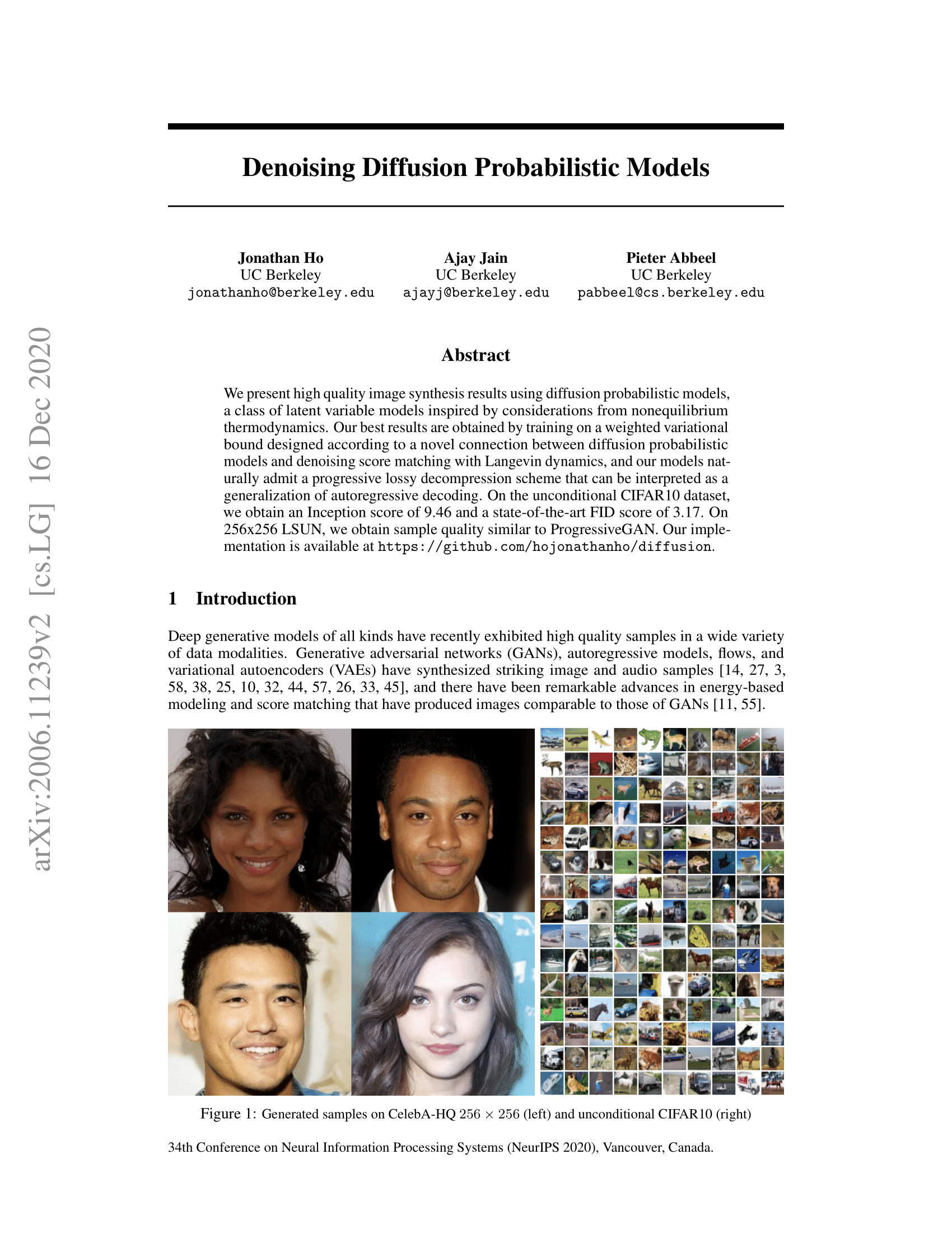

We'll install and import the required libraries first (assuming you have PyTorch installed).

中文：假设你已经安装了 [PyTorch]，我们先安装并导入必要的库。

# 中文注释：安装依赖并导入数学、可视化和张量工具
!pip install -q -U einops datasets matplotlib tqdm

import math
from inspect import isfunction
from functools import partial

%matplotlib inline
import matplotlib.pyplot as plt
from tqdm.auto import tqdm
from einops import rearrange, reduce
from einops.layers.torch import Rearrange

import torch
from torch import nn, einsum
import torch.nn.functional as F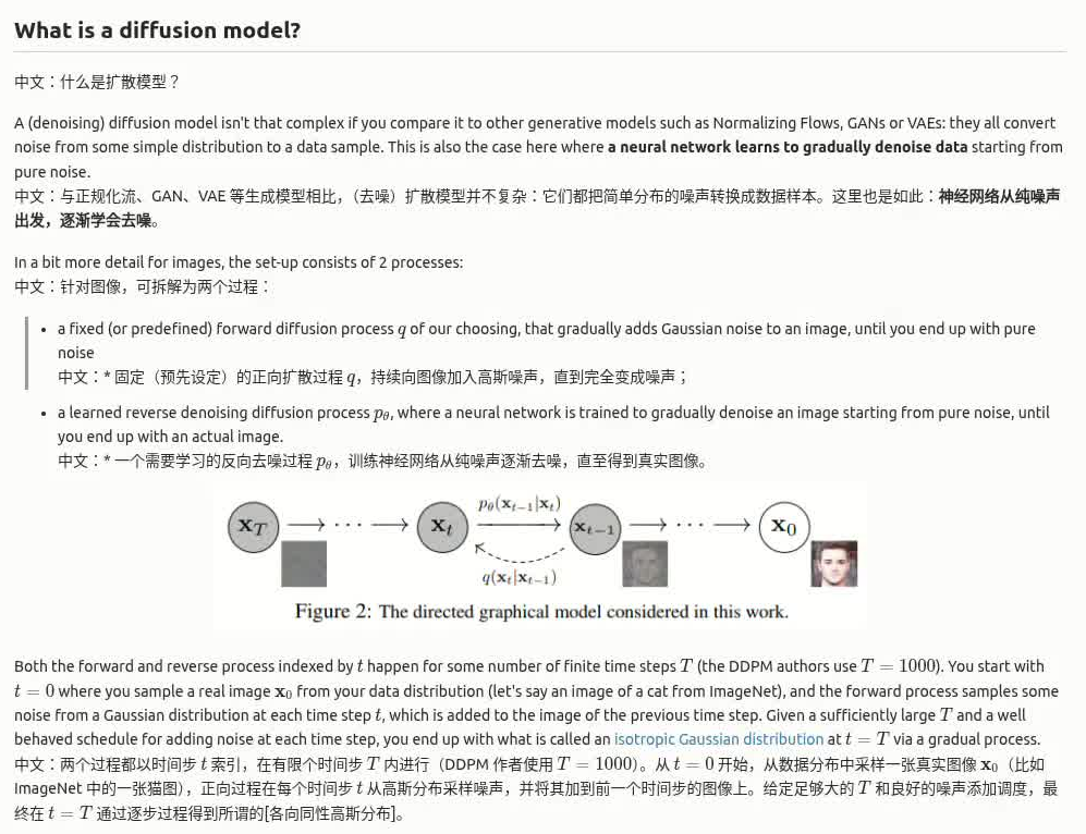

The neural network

中文：神经网络

The neural network needs to take in a noised image at a particular time step and return the predicted noise. Note that the predicted noise is a tensor that has the same size/resolution as the input image. So technically, the network takes in and outputs tensors of the same shape. What type of neural network can we use for this?

中文：神经网络要在特定时间步接收被加噪的图像，并输出预测噪声。预测噪声张量与输入图像大小一致，因此网络的输入/输出张量形状相同。那我们该用什么类型的网络呢？

What is typically used here is very similar to that of an Autoencoder, which you may remember from typical "intro to deep learning" tutorials. Autoencoders have a so-called "bottleneck" layer in between the encoder and decoder. The encoder first encodes an image into a smaller hidden representation called the "bottleneck", and the decoder then decodes that hidden representation back into an actual image. This forces the network to only keep the most important information in the bottleneck layer.

中文：常见的选择与[自编码器]十分相似------入门深度学习教程里经常出现。自编码器在编码器与解码器之间有一个"瓶颈"层：编码器把图像压缩成瓶颈表示，再由解码器还原回图像。这样可以迫使网络仅保留关键信息。

In terms of architecture, the DDPM authors went for a U-Net , introduced by (Ronneberger et al., 2015) (which, at the time, achieved state-of-the-art results for medical image segmentation). This network, like any autoencoder, consists of a bottleneck in the middle that makes sure the network learns only the most important information. Importantly, it introduced residual connections between the encoder and decoder, greatly improving gradient flow (inspired by ResNet in He et al., 2015).

中文：结构上，DDPM 采用 U-Net（由 [Ronneberger 等人, 2015] 提出，当时在医学图像分割上达到 SOTA）。与自编码器一样，它在中间也有瓶颈层确保只保留重要信息，并引入了编码器与解码器之间的残差连接，极大改善梯度流（受 [He 等人, 2015] 的 ResNet 启发）。

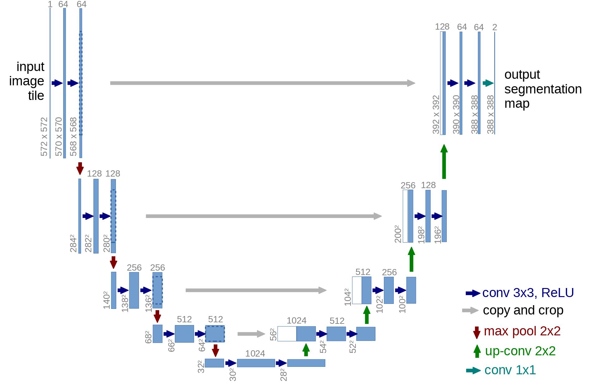
As can be seen, a U-Net model first downsamples the input (i.e. makes the input smaller in terms of spatial resolution), after which upsampling is performed.

中文：如图所示，U-Net 先对输入下采样（降低空间分辨率），然后再上采样。

Below, we implement this network, step-by-step.

中文：下面我们将一步步实现该网络。

Network helpers

中文：网络辅助函数

First, we define some helper functions and classes which will be used when implementing the neural network. Importantly, we define a Residual module, which simply adds the input to the output of a particular function (in other words, adds a residual connection to a particular function).

中文：首先定义一些工具函数和类，便于实现网络。其中 Residual 模块会把输入加到函数输出上，即向该函数添加残差连接。

We also define aliases for the up- and downsampling operations.

中文：同时给上采样与下采样操作提供别名。

# 中文注释：常用工具与残差封装
def exists(x):
    return x is not None

def default(val, d):
    if exists(val):
        return val
    return d() if isfunction(d) else d

def num_to_groups(num, divisor):
    groups = num // divisor
    remainder = num % divisor
    arr = [divisor] * groups
    if remainder > 0:
        arr.append(remainder)
    return arr

class Residual(nn.Module):
    def __init__(self, fn):
        super().__init__()
        self.fn = fn

    def forward(self, x, *args, **kwargs):
        return self.fn(x, *args, **kwargs) + x

def Upsample(dim, dim_out=None):
    return nn.Sequential(
        nn.Upsample(scale_factor=2, mode="nearest"),
        nn.Conv2d(dim, default(dim_out, dim), 3, padding=1),
    )

def Downsample(dim, dim_out=None):
    # 中文注释：PixelShuffle 风格重排作为下采样
    return nn.Sequential(
        Rearrange("b c (h p1) (w p2) -> b (c p1 p2) h w", p1=2, p2=2),
        nn.Conv2d(dim * 4, default(dim_out, dim), 1),
    )

Position embeddings

中文：时间位置嵌入

As the parameters of the neural network are shared across time (noise level), the authors employ sinusoidal position embeddings to encode ,inspiredbytheTransformer([Vaswanietal.,2017](https://arxiv.org/abs/1706.03762)).Thismakestheneuralnetwork"know"atwhichparticulartimestep(noiselevel)itisoperating,foreveryimageinabatch.

中文：由于网络参数在不同时间步（噪声级别）间共享，作者借鉴Transformer（[Vaswani等人,2017]）使用正弦位置嵌入来编码,inspiredbytheTransformer([Vaswanietal.,2017](https://arxiv.org/abs/1706.03762)).Thismakestheneuralnetwork"know"atwhichparticulartimestep(noiselevel)itisoperating,foreveryimageinabatch.

中文：由于网络参数在不同时间步（噪声级别）间共享，作者借鉴Transformer（[Vaswani等人,2017]）使用正弦位置嵌入来编码，让网络知道自己当前处理的是哪个时间步/噪声级别。

The SinusoidalPositionEmbeddings module takes a tensor of shape (batch_size, 1) as input (i.e. the noise levels of several noisy images in a batch), and turns this into a tensor of shape (batch_size, dim), with dim being the dimensionality of the position embeddings. This is then added to each residual block, as we will see further.

中文：SinusoidalPositionEmbeddings 模块输入形状为 (batch_size, 1)（即 batch 中噪声级别），输出 (batch_size, dim)，其中 dim 是嵌入维度。后续会把它加到各个残差块中。

# 中文注释：正弦时间嵌入，让网络感知噪声级别
class SinusoidalPositionEmbeddings(nn.Module):
    def __init__(self, dim):
        super().__init__()
        self.dim = dim

    def forward(self, time):
        device = time.device
        half_dim = self.dim // 2
        embeddings = math.log(10000) / (half_dim - 1)
        embeddings = torch.exp(torch.arange(half_dim, device=device) * -embeddings)
        embeddings = time[:, None] * embeddings[None, :]
        embeddings = torch.cat((embeddings.sin(), embeddings.cos()), dim=-1)
        return embeddings

ResNet block

中文：ResNet 基础块

Next, we define the core building block of the U-Net model. The DDPM authors employed a Wide ResNet block (Zagoruyko et al., 2016), but Phil Wang has replaced the standard convolutional layer by a "weight standardized" version, which works better in combination with group normalization (see (Kolesnikov et al., 2019) for details).

中文：接着定义 U-Net 的核心结构块。DDPM 使用 Wide ResNet 块（[Zagoruyko 等人, 2016]），但 Phil Wang 将标准卷积替换为"权重标准化"版本，更适合与组归一化搭配（详见 [Kolesnikov 等人, 2019]）。

# 中文注释：实现权重标准化卷积与残差块
class WeightStandardizedConv2d(nn.Conv2d):
    """
    https://arxiv.org/abs/1903.10520
    weight standardization purportedly works synergistically with group normalization
    """

    def forward(self, x):
        eps = 1e-5 if x.dtype == torch.float32 else 1e-3

        weight = self.weight
        mean = reduce(weight, "o ... -> o 1 1 1", "mean")
        var = reduce(weight, "o ... -> o 1 1 1", partial(torch.var, unbiased=False))
        normalized_weight = (weight - mean) * (var + eps).rsqrt()

        return F.conv2d(
            x,
            normalized_weight,
            self.bias,
            self.stride,
            self.padding,
            self.dilation,
            self.groups,
        )

class Block(nn.Module):
    def __init__(self, dim, dim_out, groups=8):
        super().__init__()
        self.proj = WeightStandardizedConv2d(dim, dim_out, 3, padding=1)
        self.norm = nn.GroupNorm(groups, dim_out)
        self.act = nn.SiLU()

    def forward(self, x, scale_shift=None):
        x = self.proj(x)
        x = self.norm(x)

        if exists(scale_shift):
            scale, shift = scale_shift
            x = x * (scale + 1) + shift

        x = self.act(x)
        return x

class ResnetBlock(nn.Module):
    """https://arxiv.org/abs/1512.03385"""

    def __init__(self, dim, dim_out, *, time_emb_dim=None, groups=8):
        super().__init__()
        self.mlp = (
            nn.Sequential(nn.SiLU(), nn.Linear(time_emb_dim, dim_out * 2))
            if exists(time_emb_dim)
            else None
        )

        self.block1 = Block(dim, dim_out, groups=groups)
        self.block2 = Block(dim_out, dim_out, groups=groups)
        self.res_conv = nn.Conv2d(dim, dim_out, 1) if dim != dim_out else nn.Identity()

    def forward(self, x, time_emb=None):
        scale_shift = None
        if exists(self.mlp) and exists(time_emb):
            time_emb = self.mlp(time_emb)
            time_emb = rearrange(time_emb, "b c -> b c 1 1")
            scale_shift = time_emb.chunk(2, dim=1)

        h = self.block1(x, scale_shift=scale_shift)
        h = self.block2(h)
        return h + self.res_conv(x)

Attention module

中文：注意力模块

Next, we define the attention module, which the DDPM authors added in between the convolutional blocks. Attention is the building block of the famous Transformer architecture (Vaswani et al., 2017), which has shown great success in various domains of AI, from NLP and vision to protein folding. Phil Wang employs 2 variants of attention: one is regular multi-head self-attention (as used in the Transformer), the other one is a linear attention variant (Shen et al., 2018), whose time- and memory requirements scale linear in the sequence length, as opposed to quadratic for regular attention.

中文：接着定义注意力模块，DDPM 在卷积块之间加入了它。注意力是知名 Transformer 架构的核心（[Vaswani 等人, 2017]），已在 NLP、视觉甚至[蛋白质折叠]等领域取得成功。Phil Wang 使用两种注意力：一种是 Transformer 式的多头自注意力；另一种是[线性注意力变体]（[Shen 等人, 2018]），其时间/内存复杂度对序列长度呈线性，而常规注意力是二次。

# 中文注释：常规多头自注意力
class Attention(nn.Module):
    def __init__(self, dim, heads=4, dim_head=32):
        super().__init__()
        self.scale = dim_head**-0.5
        self.heads = heads
        hidden_dim = dim_head * heads
        self.to_qkv = nn.Conv2d(dim, hidden_dim * 3, 1, bias=False)
        self.to_out = nn.Conv2d(hidden_dim, dim, 1)

    def forward(self, x):
        b, c, h, w = x.shape
        qkv = self.to_qkv(x).chunk(3, dim=1)
        q, k, v = map(
            lambda t: rearrange(t, "b (h c) x y -> b h c (x y)", h=self.heads), qkv
        )
        q = q * self.scale

        sim = einsum("b h d i, b h d j -> b h i j", q, k)
        sim = sim - sim.amax(dim=-1, keepdim=True).detach()
        attn = sim.softmax(dim=-1)

        out = einsum("b h i j, b h d j -> b h i d", attn, v)
        out = rearrange(out, "b h (x y) d -> b (h d) x y", x=h, y=w)
        return self.to_out(out)

# 中文注释：线性注意力变体
class LinearAttention(nn.Module):
    def __init__(self, dim, heads=4, dim_head=32):
        super().__init__()
        self.scale = dim_head**-0.5
        self.heads = heads
        hidden_dim = dim_head * heads
        self.to_qkv = nn.Conv2d(dim, hidden_dim * 3, 1, bias=False)

        self.to_out = nn.Sequential(nn.Conv2d(hidden_dim, dim, 1), 
                                    nn.GroupNorm(1, dim))

    def forward(self, x):
        b, c, h, w = x.shape
        qkv = self.to_qkv(x).chunk(3, dim=1)
        q, k, v = map(
            lambda t: rearrange(t, "b (h c) x y -> b h c (x y)", h=self.heads), qkv
        )

        q = q.softmax(dim=-2)
        k = k.softmax(dim=-1)

        q = q * self.scale
        context = torch.einsum("b h d n, b h e n -> b h d e", k, v)

        out = torch.einsum("b h d e, b h d n -> b h e n", context, q)
        out = rearrange(out, "b h c (x y) -> b (h c) x y", h=self.heads, x=h, y=w)
        return self.to_out(out)

Group normalization

中文：组归一化

The DDPM authors interleave the convolutional/attention layers of the U-Net with group normalization (Wu et al., 2018). Below, we define a PreNorm class, which will be used to apply groupnorm before the attention layer, as we'll see further. Note that there's been a debate about whether to apply normalization before or after attention in Transformers.

中文：DDPM 在 U-Net 的卷积/注意力层之间插入了组归一化（[Wu 等人, 2018]）。下面的 PreNorm 类会在注意力之前应用 groupnorm。值得一提的是，Transformer 中关于注意力前后归一化的顺序也有[一些讨论]。

# 中文注释：注意力前的组归一化封装
class PreNorm(nn.Module):
    def __init__(self, dim, fn):
        super().__init__()
        self.fn = fn
        self.norm = nn.GroupNorm(1, dim)

    def forward(self, x):
        x = self.norm(x)
        return self.fn(x)

Conditional U-Net

中文：条件 U-Net

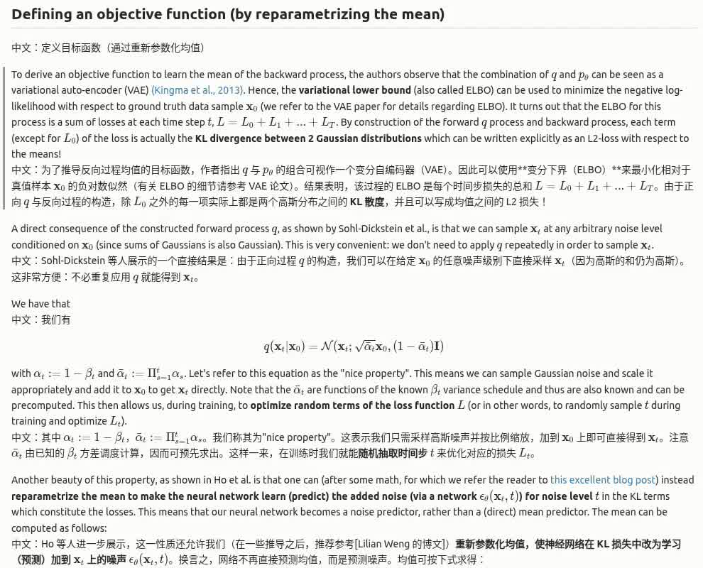
Now that we've defined all building blocks (position embeddings, ResNet blocks, attention and group normalization), it's time to define the entire neural network. Recall that the job of the network $mathbf{x}_t, t)) is to take in a batch of noisy images and their respective noise levels, and output the noise added to the input. More formally:

中文：既然已经定义了时间嵌入、ResNet 块、注意力、组归一化等组件，接下来拼装完整网络。回顾一下，$mathbf{x}_t, t)) 的工作是接收一批噪声图像及其噪声级别，并输出对应的噪声。形式化描述如下：

• the network takes a batch of noisy images of shape (batch_size, num_channels, height, width) and a batch of noise levels of shape (batch_size, 1) as input, and returns a tensor of shape (batch_size, num_channels, height, width)
  中文：* 网络输入为 (batch_size, num_channels, height, width) 的噪声图像，以及 (batch_size, 1) 的噪声级别；输出与输入图像形状一致。

The network is built up as follows:

中文：网络结构如下：

• first, a convolutional layer is applied on the batch of noisy images, and position embeddings are computed for the noise levels

  中文：* 先对噪声图像做一次卷积，并计算噪声级别的时间嵌入；

• next, a sequence of downsampling stages are applied. Each downsampling stage consists of 2 ResNet blocks + groupnorm + attention + residual connection + a downsample operation

  中文：* 接着是一系列下采样阶段：每个阶段包含 2 个 ResNet 块 + groupnorm + 注意力 + 残差 + 下采样；

• at the middle of the network, again ResNet blocks are applied, interleaved with attention

  中文：* 在网络中部，再次堆叠 ResNet 块并插入注意力；

• next, a sequence of upsampling stages are applied. Each upsampling stage consists of 2 ResNet blocks + groupnorm + attention + residual connection + an upsample operation

  中文：* 然后是一系列上采样阶段：同样由 2 个 ResNet 块 + groupnorm + 注意力 + 残差 + 上采样组成；

• finally, a ResNet block followed by a convolutional layer is applied.

  中文：* 最后通过一个 ResNet 块和卷积层输出结果。

Ultimately, neural networks stack up layers as if they were lego blocks (but it's important to understand how they work).

中文：总体来说，神经网络就像乐高一样堆叠层，但理解其原理也非常重要。

# 中文注释：完整 U-Net，包含时间嵌入及自条件支持
class Unet(nn.Module):
    def __init__(
        self,
        dim,
        init_dim=None,
        out_dim=None,
        dim_mults=(1, 2, 4, 8),
        channels=3,
        self_condition=False,
        resnet_block_groups=4,
    ):
        super().__init__()

        # determine dimensions
        self.channels = channels
        self.self_condition = self_condition
        input_channels = channels * (2 if self_condition else 1)

        init_dim = default(init_dim, dim)
        self.init_conv = nn.Conv2d(input_channels, init_dim, 1, padding=0) # changed to 1 and 0 from 7,3

        dims = [init_dim, *map(lambda m: dim * m, dim_mults)]
        in_out = list(zip(dims[:-1], dims[1:]))

        block_klass = partial(ResnetBlock, groups=resnet_block_groups)

        # time embeddings
        time_dim = dim * 4

        self.time_mlp = nn.Sequential(
            SinusoidalPositionEmbeddings(dim),
            nn.Linear(dim, time_dim),
            nn.GELU(),
            nn.Linear(time_dim, time_dim),
        )

        # layers
        self.downs = nn.ModuleList([])
        self.ups = nn.ModuleList([])
        num_resolutions = len(in_out)

        for ind, (dim_in, dim_out) in enumerate(in_out):
            is_last = ind >= (num_resolutions - 1)

            self.downs.append(
                nn.ModuleList(
                    [
                        block_klass(dim_in, dim_in, time_emb_dim=time_dim),
                        block_klass(dim_in, dim_in, time_emb_dim=time_dim),
                        Residual(PreNorm(dim_in, LinearAttention(dim_in))),
                        Downsample(dim_in, dim_out)
                        if not is_last
                        else nn.Conv2d(dim_in, dim_out, 3, padding=1),
                    ]
                )
            )

        mid_dim = dims[-1]
        self.mid_block1 = block_klass(mid_dim, mid_dim, time_emb_dim=time_dim)
        self.mid_attn = Residual(PreNorm(mid_dim, Attention(mid_dim)))
        self.mid_block2 = block_klass(mid_dim, mid_dim, time_emb_dim=time_dim)

        for ind, (dim_in, dim_out) in enumerate(reversed(in_out)):
            is_last = ind == (len(in_out) - 1)

            self.ups.append(
                nn.ModuleList(
                    [
                        block_klass(dim_out + dim_in, dim_out, time_emb_dim=time_dim),
                        block_klass(dim_out + dim_in, dim_out, time_emb_dim=time_dim),
                        Residual(PreNorm(dim_out, LinearAttention(dim_out))),
                        Upsample(dim_out, dim_in)
                        if not is_last
                        else nn.Conv2d(dim_out, dim_in, 3, padding=1),
                    ]
                )
            )

        self.out_dim = default(out_dim, channels)

        self.final_res_block = block_klass(dim * 2, dim, time_emb_dim=time_dim)
        self.final_conv = nn.Conv2d(dim, self.out_dim, 1)

    def forward(self, x, time, x_self_cond=None):
        if self.self_condition:
            x_self_cond = default(x_self_cond, lambda: torch.zeros_like(x))
            x = torch.cat((x_self_cond, x), dim=1)

        x = self.init_conv(x)
        r = x.clone()

        t = self.time_mlp(time)

        h = []

        for block1, block2, attn, downsample in self.downs:
            x = block1(x, t)
            h.append(x)

            x = block2(x, t)
            x = attn(x)
            h.append(x)

            x = downsample(x)

        x = self.mid_block1(x, t)
        x = self.mid_attn(x)
        x = self.mid_block2(x, t)

        for block1, block2, attn, upsample in self.ups:
            x = torch.cat((x, h.pop()), dim=1)
            x = block1(x, t)

            x = torch.cat((x, h.pop()), dim=1)
            x = block2(x, t)
            x = attn(x)

            x = upsample(x)

        x = torch.cat((x, r), dim=1)

        x = self.final_res_block(x, t)
        return self.final_conv(x)

Defining the forward diffusion process

中文：定义正向扩散过程

The forward diffusion process gradually adds noise to an image from the real distribution, in a number of time steps .Thishappensaccordingtoa∗∗varianceschedule∗∗.TheoriginalDDPMauthorsemployedalinearschedule:中文：正向扩散过程会在.Thishappensaccordingtoa∗∗varianceschedule∗∗.TheoriginalDDPMauthorsemployedalinearschedule:中文：正向扩散过程会在 个时间步内逐步向真实图像添加噪声。它依据方差调度进行。DDPM 原论文使用线性调度：

We set the forward process variances to constants increasing linearly from .中文：>将正向过程的方差线性递增，起点.中文：>将正向过程的方差线性递增，起点。

However, it was shown in (Nichol et al., 2021) that better results can be achieved when employing a cosine schedule.

中文：不过 ([Nichol 等人, 2021]) 指出，采用余弦调度的效果更好。

Below, we define various schedules for the timesteps(we′llchooseonelateron).中文：下面为timesteps(we′llchooseonelateron).中文：下面为 个时间步定义多种调度（稍后会选择其一）。

# 中文注释：多种 beta 调度函数
def cosine_beta_schedule(timesteps, s=0.008):
    """
    cosine schedule as proposed in https://arxiv.org/abs/2102.09672
    """
    steps = timesteps + 1
    x = torch.linspace(0, timesteps, steps)
    alphas_cumprod = torch.cos(((x / timesteps) + s) / (1 + s) * torch.pi * 0.5) ** 2
    alphas_cumprod = alphas_cumprod / alphas_cumprod[0]
    betas = 1 - (alphas_cumprod[1:] / alphas_cumprod[:-1])
    return torch.clip(betas, 0.0001, 0.9999)

def linear_beta_schedule(timesteps):
    beta_start = 0.0001
    beta_end = 0.02
    return torch.linspace(beta_start, beta_end, timesteps)

def quadratic_beta_schedule(timesteps):
    beta_start = 0.0001
    beta_end = 0.02
    return torch.linspace(beta_start**0.5, beta_end**0.5, timesteps) ** 2

def sigmoid_beta_schedule(timesteps):
    beta_start = 0.0001
    beta_end = 0.02
    betas = torch.linspace(-6, 6, timesteps)
    return torch.sigmoid(betas) * (beta_end - beta_start) + beta_start

To start with, let's use the linear schedule for indexforabatchofindices.中文：首先以indexforabatchofindices.中文：首先以。

# 中文注释：根据 beta 预计算一系列辅助张量
timesteps = 300

# define beta schedule
betas = linear_beta_schedule(timesteps=timesteps)

# define alphas 
alphas = 1. - betas
alphas_cumprod = torch.cumprod(alphas, axis=0)
alphas_cumprod_prev = F.pad(alphas_cumprod[:-1], (1, 0), value=1.0)
sqrt_recip_alphas = torch.sqrt(1.0 / alphas)

# calculations for diffusion q(x_t | x_{t-1}) and others
sqrt_alphas_cumprod = torch.sqrt(alphas_cumprod)
sqrt_one_minus_alphas_cumprod = torch.sqrt(1. - alphas_cumprod)

# calculations for posterior q(x_{t-1} | x_t, x_0)
posterior_variance = betas * (1. - alphas_cumprod_prev) / (1. - alphas_cumprod)

def extract(a, t, x_shape):
    batch_size = t.shape[0]
    out = a.gather(-1, t.cpu())
    return out.reshape(batch_size, *((1,) * (len(x_shape) - 1))).to(t.device)

We'll illustrate with a cats image how noise is added at each time step of the diffusion process.

中文：下面以一张猫的图像演示扩散过程中各时间步的加噪效果。

# 中文注释：下载示例图像并读取
from PIL import Image
import requests

url = 'http://images.cocodataset.org/val2017/000000039769.jpg'
image = Image.open(requests.get(url, stream=True).raw) # PIL image of shape HWC
image

Noise is added to PyTorch tensors, rather than Pillow Images. We'll first define image transformations that allow us to go from a PIL image to a PyTorch tensor (on which we can add the noise), and vice versa.

中文：噪声会加在 PyTorch 张量上，而不是 PIL 图像上。我们先定义图像变换，将 PIL 图像转成张量（便于加噪），以及反向变换。

These transformations are fairly simple: we first normalize images by dividing by range),andthenmakesuretheyareintherange),andthenmakesuretheyareinthe range. From the DDPM paper:

中文：这些变换很简单：先将图像除以 255 归一化到 $。DDPM 论文中写道：

We assume that image data consists of integers in $mathbf{x}_T)).

中文：> 假设图像数据来自 $mathbf{x}_T)) 开始时输入尺度一致。

# 中文注释：构建张量化与反向变换
from torchvision.transforms import Compose, ToTensor, Lambda, ToPILImage, CenterCrop, Resize

image_size = 128
transform = Compose([
    Resize(image_size),
    CenterCrop(image_size),
    ToTensor(), # turn into torch Tensor of shape CHW, divide by 255
    Lambda(lambda t: (t * 2) - 1),
    
])

x_start = transform(image).unsqueeze(0)
x_start.shape

We also define the reverse transform, which takes in a PyTorch tensor containing values in andturnthembackintoaPILimage:中文：再定义逆变换，把andturnthembackintoaPILimage:中文：再定义逆变换，把 范围的张量还原成 PIL 图像：

# 中文注释：逆变换，将张量还原为 PIL
import numpy as np

reverse_transform = Compose([
     Lambda(lambda t: (t + 1) / 2),
     Lambda(lambda t: t.permute(1, 2, 0)), # CHW to HWC
     Lambda(lambda t: t * 255.),
     Lambda(lambda t: t.numpy().astype(np.uint8)),
     ToPILImage(),
])

Let's verify this:

中文：验证一下：

reverse_transform(x_start.squeeze())

We can now define the forward diffusion process as in the paper:

中文：现在按照论文定义正向扩散过程：

# 中文注释：利用 nice property 实现前向采样
def q_sample(x_start, t, noise=None):
    if noise is None:
        noise = torch.randn_like(x_start)

    sqrt_alphas_cumprod_t = extract(sqrt_alphas_cumprod, t, x_start.shape)
    sqrt_one_minus_alphas_cumprod_t = extract(
        sqrt_one_minus_alphas_cumprod, t, x_start.shape
    )

    return sqrt_alphas_cumprod_t * x_start + sqrt_one_minus_alphas_cumprod_t * noise

Let's test it on a particular time step:

中文：在某个时间步上测试：

def get_noisy_image(x_start, t):
  # add noise
  x_noisy = q_sample(x_start, t=t)

  # turn back into PIL image
  noisy_image = reverse_transform(x_noisy.squeeze())

  return noisy_image

# 中文注释：查看 t=40 的加噪效果
t = torch.tensor([40])

get_noisy_image(x_start, t)

Let's visualize this for various time steps:

中文：再看看多个时间步的对比：

# 中文注释：绘制不同时间步下的噪声图
import matplotlib.pyplot as plt

# use seed for reproducability
torch.manual_seed(0)

# source: https://pytorch.org/vision/stable/auto_examples/plot_transforms.html#sphx-glr-auto-examples-plot-transforms-py
def plot(imgs, with_orig=False, row_title=None, **imshow_kwargs):
    if not isinstance(imgs[0], list):
        # Make a 2d grid even if there's just 1 row
        imgs = [imgs]

    num_rows = len(imgs)
    num_cols = len(imgs[0]) + with_orig
    fig, axs = plt.subplots(figsize=(200,200), nrows=num_rows, ncols=num_cols, squeeze=False)
    for row_idx, row in enumerate(imgs):
        row = [image] + row if with_orig else row
        for col_idx, img in enumerate(row):
            ax = axs[row_idx, col_idx]
            ax.imshow(np.asarray(img), **imshow_kwargs)
            ax.set(xticklabels=[], yticklabels=[], xticks=[], yticks=[])

    if with_orig:
        axs[0, 0].set(title='Original image')
        axs[0, 0].title.set_size(8)
    if row_title is not None:
        for row_idx in range(num_rows):
            axs[row_idx, 0].set(ylabel=row_title[row_idx])

    plt.tight_layout()

plot([get_noisy_image(x_start, torch.tensor([t])) for t in [0, 50, 100, 150, 199]])

This means that we can now define the loss function given the model as follows:

中文：这就可以配合模型定义损失函数：

# 中文注释：根据噪声预测选择 L1/L2/Huber 损失
def p_losses(denoise_model, x_start, t, noise=None, loss_type="l1"):
    if noise is None:
        noise = torch.randn_like(x_start)

    x_noisy = q_sample(x_start=x_start, t=t, noise=noise)
    predicted_noise = denoise_model(x_noisy, t)

    if loss_type == 'l1':
        loss = F.l1_loss(noise, predicted_noise)
    elif loss_type == 'l2':
        loss = F.mse_loss(noise, predicted_noise)
    elif loss_type == "huber":
        loss = F.smooth_l1_loss(noise, predicted_noise)
    else:
        raise NotImplementedError()

    return loss

The denoise_model will be our U-Net defined above. We'll employ the Huber loss between the true and the predicted noise.

中文：denoise_model 就是上面定义的 U-Net。这里采用真实噪声与预测噪声之间的 Huber 损失。

Define a PyTorch Dataset + DataLoader

中文：定义 PyTorch Dataset 与 DataLoader

Here we define a regular PyTorch Dataset. The dataset simply consists of images from a real dataset, like Fashion-MNIST, CIFAR-10 or ImageNet, scaled linearly to .中文：下面定义常规[PyTorchDataset]。数据集可以是Fashion−MNIST、CIFAR−10、ImageNet等真实图像，并线性缩放到.中文：下面定义常规[PyTorchDataset]。数据集可以是Fashion−MNIST、CIFAR−10、ImageNet等真实图像，并线性缩放到。

Each image is resized to the same size. Interesting to note is that images are also randomly horizontally flipped. From the paper:

中文：所有图像都会调整为同一尺寸，并进行随机水平翻转。论文写道：

We used random horizontal flips during training for CIFAR10; we tried training both with and without flips, and found flips to improve sample quality slightly.

中文：> 在 CIFAR10 训练中我们使用了随机水平翻转；测试发现开启翻转能略微提升样本质量。

Here we use the 🤗 Datasets library to easily load the Fashion MNIST dataset from the hub. This dataset consists of images which already have the same resolution, namely 28x28.

中文：这里借助 🤗 [Datasets 库] 从 [Hub] 载入 Fashion-MNIST。该数据集本身就是 28x28 分辨率。

# 中文注释：加载 Fashion-MNIST 数据集
from datasets import load_dataset

# load dataset from the hub
dataset = load_dataset("fashion_mnist")
image_size = 28
channels = 1
batch_size = 128

Next, we define a function which we'll apply on-the-fly on the entire dataset. We use the with_transform functionality for that. The function just applies some basic image preprocessing: random horizontal flips, rescaling and finally make them have values in the range.中文：接着定义一个函数，通过'withtransform'动态作用于整个数据集，实现随机水平翻转、归一化以及缩放到range.中文：接着定义一个函数，通过'witht​ransform'动态作用于整个数据集，实现随机水平翻转、归一化以及缩放到。

# 中文注释：构建数据增强与 DataLoader
from torchvision import transforms
from torch.utils.data import DataLoader

# define image transformations (e.g. using torchvision)
transform = Compose([
            transforms.RandomHorizontalFlip(),
            transforms.ToTensor(),
            transforms.Lambda(lambda t: (t * 2) - 1)
])

# define function
def transforms_fn(examples):
   examples["pixel_values"] = [transform(image.convert("L")) for image in examples["image"]]
   del examples["image"]

   return examples

transformed_dataset = dataset.with_transform(transforms_fn).remove_columns("label")

# create dataloader
dataloader = DataLoader(transformed_dataset["train"], batch_size=batch_size, shuffle=True)

batch = next(iter(dataloader))
print(batch.keys())

Sampling

中文：采样

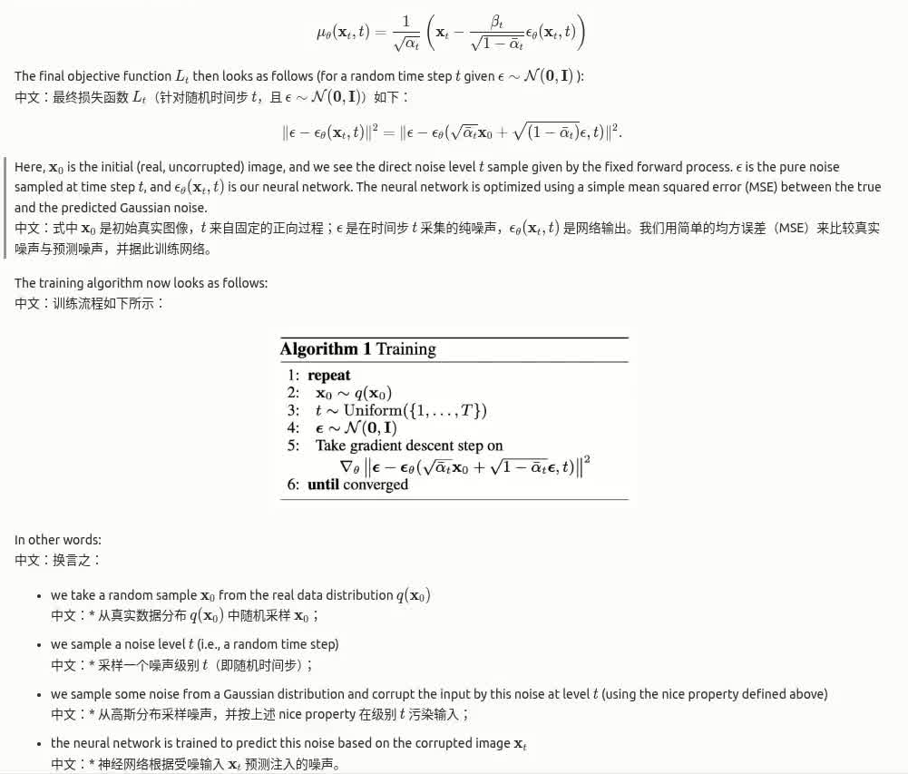
As we'll sample from the model during training (in order to track progress), we define the code for that below. Sampling is summarized in the paper as Algorithm 2:

中文：训练过程中会周期性地从模型采样以监控进展，下面给出对应代码。论文中的算法 2 对采样进行了总结：

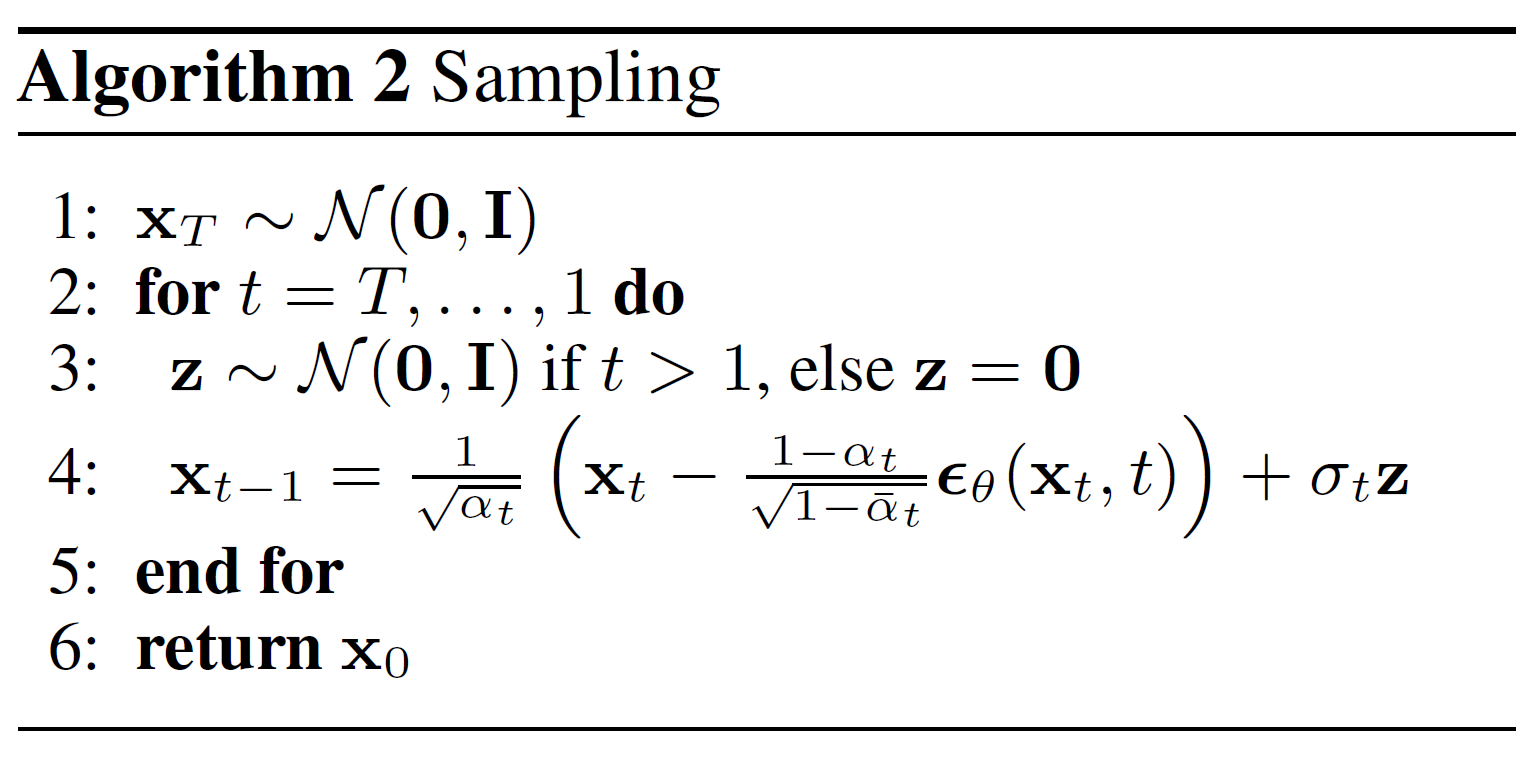
Generating new images from a diffusion model happens by reversing the diffusion process: we start from ,wherewesamplepurenoisefromaGaussiandistribution,andthenuseourneuralnetworktograduallydenoiseit(usingtheconditionalprobabilityithaslearned),untilweendupattimestep,wherewesamplepurenoisefromaGaussiandistribution,andthenuseourneuralnetworktograduallydenoiseit(usingtheconditionalprobabilityithaslearned),untilweendupattimestep by plugging in the reparametrization of the mean, using our noise predictor. Remember that the variance is known ahead of time.

中文：从扩散模型生成新图像的方式就是反向扩散：从 $。方差在前面已经预先计算。

Ideally, we end up with an image that looks like it came from the real data distribution.

中文：理想情况下，最终得到的图像看起来就像来自真实数据分布。

The code below implements this.

中文：以下即为实现。

# 中文注释：实现反向采样（算法2）
@torch.no_grad()
def p_sample(model, x, t, t_index):
    betas_t = extract(betas, t, x.shape)
    sqrt_one_minus_alphas_cumprod_t = extract(
        sqrt_one_minus_alphas_cumprod, t, x.shape
    )
    sqrt_recip_alphas_t = extract(sqrt_recip_alphas, t, x.shape)
    
    # Equation 11 in the paper
    # Use our model (noise predictor) to predict the mean
    model_mean = sqrt_recip_alphas_t * (
        x - betas_t * model(x, t) / sqrt_one_minus_alphas_cumprod_t
    )

    if t_index == 0:
        return model_mean
    else:
        posterior_variance_t = extract(posterior_variance, t, x.shape)
        noise = torch.randn_like(x)
        # Algorithm 2 line 4:
        return model_mean + torch.sqrt(posterior_variance_t) * noise 

# Algorithm 2 (including returning all images)
@torch.no_grad()
def p_sample_loop(model, shape):
    device = next(model.parameters()).device

    b = shape[0]
    # start from pure noise (for each example in the batch)
    img = torch.randn(shape, device=device)
    imgs = []

    for i in tqdm(reversed(range(0, timesteps)), desc='sampling loop time step', total=timesteps):
        img = p_sample(model, img, torch.full((b,), i, device=device, dtype=torch.long), i)
        imgs.append(img.cpu().numpy())
    return imgs

@torch.no_grad()
def sample(model, image_size, batch_size=16, channels=3):
    return p_sample_loop(model, shape=(batch_size, channels, image_size, image_size))

Note that the code above is a simplified version of the original implementation. We found our simplification (which is in line with Algorithm 2 in the paper) to work just as well as the original, more complex implementation, which employs clipping.

中文：注意，上述代码是原实现的简化版，与论文算法 2 一致，实践中效果也很好；相比之下，[原始实现] 更复杂，还引入了[clipping]。

Train the model

中文：训练模型

Next, we train the model in regular PyTorch fashion. We also define some logic to periodically save generated images, using the sample method defined above.

中文：接下来以常规 PyTorch 方式训练模型，并利用前面 sample 函数定期保存生成图像。

# 中文注释：准备结果保存目录与调度
from pathlib import Path

def num_to_groups(num, divisor):
    groups = num // divisor
    remainder = num % divisor
    arr = [divisor] * groups
    if remainder > 0:
        arr.append(remainder)
    return arr

results_folder = Path("./results")
results_folder.mkdir(exist_ok = True)
save_and_sample_every = 1000

Below, we define the model, and move it to the GPU. We also define a standard optimizer (Adam).

中文：下面实例化模型并移到 GPU，同时设置 Adam 优化器。

# 中文注释：初始化 U-Net 与优化器
from torch.optim import Adam

device = "cuda" if torch.cuda.is_available() else "cpu"

model = Unet(
    dim=image_size,
    channels=channels,
    dim_mults=(1, 2, 4,)
)
model.to(device)

optimizer = Adam(model.parameters(), lr=1e-3)

Let's start training!

中文：开始训练！

# 中文注释：主训练循环
from torchvision.utils import save_image

epochs = 6

for epoch in range(epochs):
    for step, batch in enumerate(dataloader):
      optimizer.zero_grad()

      batch_size = batch["pixel_values"].shape[0]
      batch = batch["pixel_values"].to(device)

      # Algorithm 1 line 3: sample t uniformally for every example in the batch
      t = torch.randint(0, timesteps, (batch_size,), device=device).long()

      loss = p_losses(model, batch, t, loss_type="huber")

      if step % 100 == 0:
        print("Loss:", loss.item())

      loss.backward()
      optimizer.step()

      # save generated images
      if step != 0 and step % save_and_sample_every == 0:
        milestone = step // save_and_sample_every
        batches = num_to_groups(4, batch_size)
        all_images_list = list(map(lambda n: sample(model, batch_size=n, channels=channels), batches))
        all_images = torch.cat(all_images_list, dim=0)
        all_images = (all_images + 1) * 0.5
        save_image(all_images, str(results_folder / f'sample-{milestone}.png'), nrow = 6)

Sampling (inference)

中文：推理采样

To sample from the model, we can just use our sample function defined above:

中文：推理时直接调用上面的 sample 函数：

# 中文注释：批量生成样本并展示
# sample 64 images
samples = sample(model, image_size=image_size, batch_size=64, channels=channels)

# show a random one
random_index = 5
plt.imshow(samples[-1][random_index].reshape(image_size, image_size, channels), cmap="gray")

It seems like the model is capable of generating a nice T-shirt! Keep in mind that the dataset we trained on is pretty low-resolution (28x28).

中文：看起来模型已经能生成不错的 T 恤图案！不过别忘了，训练集的分辨率只有 28x28。

We can also create a gif of the denoising process:

中文：我们还能把去噪过程做成 GIF：

# 中文注释：制作去噪过程动图
import matplotlib.animation as animation

random_index = 53

fig = plt.figure()
ims = []
for i in range(timesteps):
    im = plt.imshow(samples[i][random_index].reshape(image_size, image_size, channels), cmap="gray", animated=True)
    ims.append([im])

animate = animation.ArtistAnimation(fig, ims, interval=50, blit=True, repeat_delay=1000)
animate.save('diffusion.gif')
plt.show()

Follow-up reads

中文：后续阅读

Note that the DDPM paper showed that diffusion models are a promising direction for (un)conditional image generation. This has since then (immensely) been improved, most notably for text-conditional image generation. Below, we list some important (but far from exhaustive) follow-up works:

中文：DDPM 论文表明，扩散模型在条件/无条件图像生成方面前景广阔。此后相关工作突飞猛进，尤其是文本条件图像生成。以下列出一些重要（但远不完整）的后续研究：

• Improved Denoising Diffusion Probabilistic Models (Nichol et al., 2021): finds that learning the variance of the conditional distribution (besides the mean) helps in improving performance

  中文：- Improved Denoising Diffusion Probabilistic Models：提出同时学习方差能提升性能。

• Cascaded Diffusion Models for High Fidelity Image Generation (Ho et al., 2021): introduces cascaded diffusion, which comprises a pipeline of multiple diffusion models that generate images of increasing resolution for high-fidelity image synthesis

  中文：- Cascaded Diffusion Models for High Fidelity Image Generation：提出级联扩散，通过多模型逐级提升分辨率以产生高保真图像。

• Diffusion Models Beat GANs on Image Synthesis (Dhariwal et al., 2021): show that diffusion models can achieve image sample quality superior to the current state-of-the-art generative models by improving the U-Net architecture, as well as introducing classifier guidance

  中文：- Diffusion Models Beat GANs on Image Synthesis：通过改进 U-Net 和引入分类器引导，展现扩散模型在图像质量上超越最先进生成模型。

• Classifier-Free Diffusion Guidance (Ho et al., 2021): shows that you don't need a classifier for guiding a diffusion model by jointly training a conditional and an unconditional diffusion model with a single neural network

  中文：- Classifier-Free Diffusion Guidance：提出无需外部分类器，通过单模型联合训练条件/无条件扩散实现引导。

• Hierarchical Text-Conditional Image Generation with CLIP Latents (DALL-E 2) (Ramesh et al., 2022): uses a prior to turn a text caption into a CLIP image embedding, after which a diffusion model decodes it into an image

  中文：- Hierarchical Text-Conditional Image Generation with CLIP Latents（DALL·E 2）：用先验将文本转成 CLIP 图像嵌入，再由扩散模型解码成图像。

• Photorealistic Text-to-Image Diffusion Models with Deep Language Understanding (ImageGen) (Saharia et al., 2022): shows that combining a large pre-trained language model (e.g. T5) with cascaded diffusion works well for text-to-image synthesis

  中文：- Photorealistic Text-to-Image Diffusion Models with Deep Language Understanding（ImageGen）：结合大型预训练语言模型（如 T5）与级联扩散，可高质量实现文生图。

Note that this list only includes important works until the time of writing, which is June 7th, 2022.

中文：该列表仅涵盖截至 2022 年 6 月 7 日之前的重要工作。

For now, it seems that the main (perhaps only) disadvantage of diffusion models is that they require multiple forward passes to generate an image (which is not the case for generative models like GANs). However, there's research going on that enables high-fidelity generation in as few as 10 denoising steps.

中文：目前看来，扩散模型的主要缺点（或许也是唯一缺点）是生成一张图需要多次前向传递，而 GAN 等模型则无需如此。不过已经有[研究]在尝试把高保真生成压缩到约 10 步去噪。