import numpy as np
import matplotlib.pyplot as plt
from scipy import stats
from typing import List, Callable
import seaborn as sns
from scipy.special import comb
def true_pass_at_k(p: float, k: int) -> float:
"""True pass@k value: 1 - (1-p)^k"""
return 1 - (1 - p) ** k
def bootstrap_estimator(samples: List[bool], k: int, n_bootstrap: int = 1000) -> float:
"""Bootstrap estimator for pass@k"""
n = len(samples)
if n == 0:
return 0.0
bootstrap_estimates = []
for _ in range(n_bootstrap):
# Sample with replacement
bootstrap_sample = np.random.choice(samples, size=min(k, n), replace=True)
bootstrap_estimates.append(np.any(bootstrap_sample))
return np.mean(bootstrap_estimates)
# Set style for better plots
plt.style.use('seaborn-v0_8')
sns.set_palette("husl")
true_p = 0.3
max_samples=100
n_trials=200
k_values = [1, 3, 5, 10, 20]
# Colors for different k values
# Set up the plot
fig, axes = plt.subplots(1, 1, figsize=(15, 12))
colors = plt.cm.viridis(np.linspace(0, 1, len(k_values)))
ax = axes
for k_idx, k in enumerate(k_values):
# True value
true_value = true_pass_at_k(true_p, k)
# Store estimates for different sample sizes
sample_sizes = []
estimates_mean = []
estimates_std = []
biases = []
for n_samples in range(1, max_samples + 1, 5):
trial_estimates = []
for trial in range(n_trials):
# Generate samples
samples = np.random.binomial(1, true_p, n_samples).astype(bool)
estimate = bootstrap_estimator(samples.tolist(), k, 500)
trial_estimates.append(estimate)
sample_sizes.append(n_samples)
estimates_mean.append(np.mean(trial_estimates))
estimates_std.append(np.std(trial_estimates))
biases.append(np.mean(trial_estimates) - true_value)
# Plot mean estimates
ax.plot(sample_sizes, estimates_mean,
color=colors[k_idx], label=f'k={k}', linewidth=2)
# Add shaded region for ±1 std
ax.fill_between(sample_sizes,
np.array(estimates_mean) - np.array(estimates_std),
np.array(estimates_mean) + np.array(estimates_std),
alpha=0.2, color=colors[k_idx])
# Plot true value as horizontal line
ax.axhline(y=true_value, color=colors[k_idx], linestyle='--', alpha=0.7)
ax.set_xlabel('Number of Samples (n)')
ax.set_ylabel('pass@k Estimate')
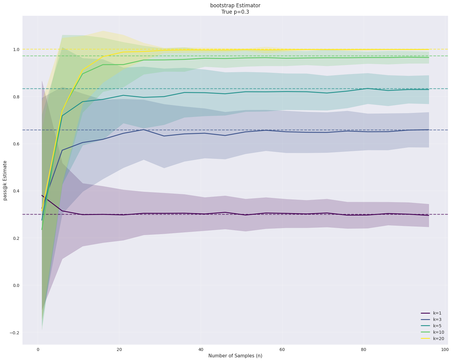
ax.set_title(f'bootstrap Estimator\n'
f'True p={true_p}')
ax.legend()
ax.grid(True, alpha=0.3)
plt.tight_layout()
plt.show()
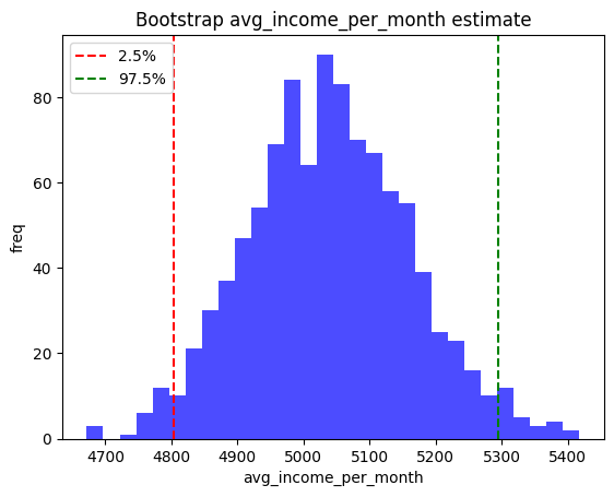
输出如下所示,在样本数n比较小的时候,方差还是比较大的。
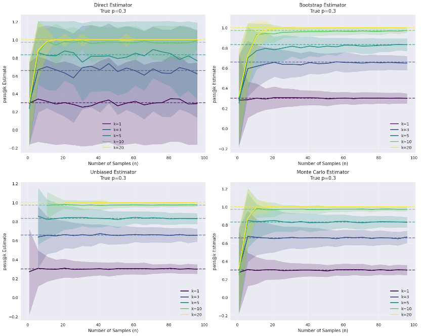
3 综合模拟对比
这里进一步对比bootstrap估计和其他估计模拟估计手段。
3.1 bootstrap
bootstrap模拟过程代码示例如下。
复制代码
def bootstrap_estimator(samples: List[bool], k: int, n_bootstrap: int = 1000) -> float:
    """Bootstrap estimator for pass@k"""
    n = len(samples)
    if n == 0:
        return 0.0

    bootstrap_estimates = []
    for _ in range(n_bootstrap):
        # Sample with replacement
        bootstrap_sample = np.random.choice(samples, size=min(k, n), replace=True)
        bootstrap_estimates.append(np.any(bootstrap_sample))

    return np.mean(bootstrap_estimates)
3.2 monte carlo
monte carlo模拟估计代码示例如下
复制代码
def monte_carlo_estimator(samples: List[bool], k: int, n_simulations: int = 1000) -> float:
    """Monte Carlo estimator for pass@k"""
    n = len(samples)
    if n == 0:
        return 0.0

    successes = 0
    for _ in range(n_simulations):
        # Randomly select k samples without replacement
        selected_indices = np.random.choice(n, size=min(k, n), replace=False)
        selected_samples = [samples[i] for i in selected_indices]
        if np.any(selected_samples):
            successes += 1

    return successes / n_simulations
3.3 直接模拟
直接模拟代码示例如下
复制代码
def direct_estimator(samples: List[bool], k: int) -> float:
    """Direct estimator using sample proportion"""
    n = len(samples)
    if n == 0:
        return 0.0

    # Take first k samples (or all if n < k)
    selected_samples = samples[:min(k, n)]
    return float(np.any(selected_samples))
3.4 unbiased模拟
无偏模拟,也就是OpenAI在HumanEval采用的模拟方法,代码示例如下
复制代码
def unbiased_estimator(samples: List[bool], k: int) -> float:
    """Unbiased estimator using combinatorial approach"""
    n = len(samples)
    if n < k:
        return float(np.any(samples))  # Fallback if not enough samples

    # Count number of successes
    c = np.sum(samples)

    if c == 0:
        return 0.0

    # Unbiased estimator: 1 - (n-c choose k) / (n choose k)
    n_choose_k = comb(n, k)
    if n - c < k:
        return 1.0

    n_minus_c_choose_k = comb(n - c, k)
    return 1 - n_minus_c_choose_k / n_choose_k
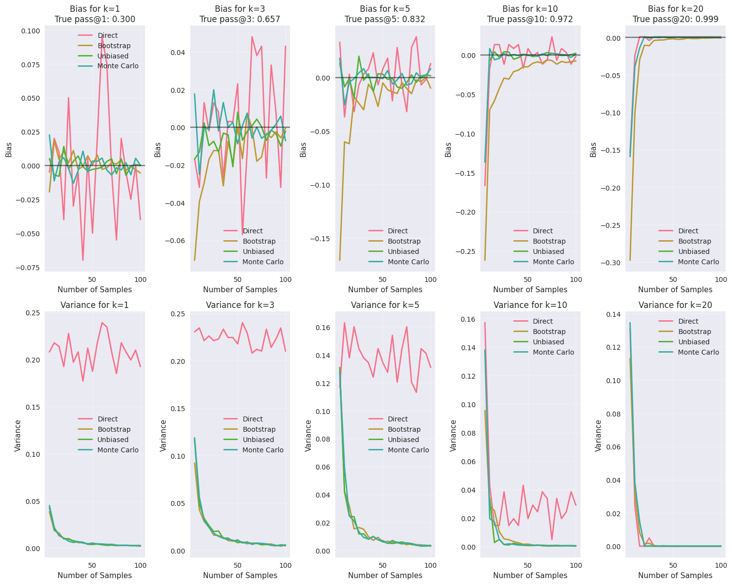
3.4 综合对比
综合以上多种模拟方案,进行对比示例。
复制代码
import numpy as np
import matplotlib.pyplot as plt
from scipy import stats
from typing import List, Callable
import seaborn as sns
from scipy.special import comb

# Set style for better plots
plt.style.use('seaborn-v0_8')
sns.set_palette("husl")

def true_pass_at_k(p: float, k: int) -> float:
    """True pass@k value: 1 - (1-p)^k"""
    return 1 - (1 - p) ** k

def bootstrap_estimator(samples: List[bool], k: int, n_bootstrap: int = 1000) -> float:
    """Bootstrap estimator for pass@k"""
    n = len(samples)
    if n == 0:
        return 0.0

    bootstrap_estimates = []
    for _ in range(n_bootstrap):
        # Sample with replacement
        bootstrap_sample = np.random.choice(samples, size=min(k, n), replace=True)
        bootstrap_estimates.append(np.any(bootstrap_sample))

    return np.mean(bootstrap_estimates)

def direct_estimator(samples: List[bool], k: int) -> float:
    """Direct estimator using sample proportion"""
    n = len(samples)
    if n == 0:
        return 0.0

    # Take first k samples (or all if n < k)
    selected_samples = samples[:min(k, n)]
    return float(np.any(selected_samples))

def unbiased_estimator(samples: List[bool], k: int) -> float:
    """Unbiased estimator using combinatorial approach"""
    n = len(samples)
    if n < k:
        return float(np.any(samples))  # Fallback if not enough samples

    # Count number of successes
    c = np.sum(samples)

    if c == 0:
        return 0.0

    # Unbiased estimator: 1 - (n-c choose k) / (n choose k)
    n_choose_k = comb(n, k)
    if n - c < k:
        return 1.0

    n_minus_c_choose_k = comb(n - c, k)
    return 1 - n_minus_c_choose_k / n_choose_k

def monte_carlo_estimator(samples: List[bool], k: int, n_simulations: int = 1000) -> float:
    """Monte Carlo estimator for pass@k"""
    n = len(samples)
    if n == 0:
        return 0.0

    successes = 0
    for _ in range(n_simulations):
        # Randomly select k samples without replacement
        selected_indices = np.random.choice(n, size=min(k, n), replace=False)
        selected_samples = [samples[i] for i in selected_indices]
        if np.any(selected_samples):
            successes += 1

    return successes / n_simulations

def analyze_estimators(true_p: float = 0.3, max_samples: int = 100, k_values: List[int] = None, n_trials: int = 100):
    """Analyze bias and variance of different pass@k estimators"""
    if k_values is None:
        k_values = [1, 3, 5, 10, 20]

    estimators = {
        'Direct': direct_estimator,
        'Bootstrap': lambda samples, k: bootstrap_estimator(samples, k, 500),
        'Unbiased': unbiased_estimator,
        'Monte Carlo': lambda samples, k: monte_carlo_estimator(samples, k, 500)
    }

    # Set up the plot
    fig, axes = plt.subplots(2, 2, figsize=(15, 12))
    axes = axes.flatten()

    # Colors for different k values
    colors = plt.cm.viridis(np.linspace(0, 1, len(k_values)))

    for idx, (estimator_name, estimator_func) in enumerate(estimators.items()):
        ax = axes[idx]

        for k_idx, k in enumerate(k_values):
            # True value
            true_value = true_pass_at_k(true_p, k)

            # Store estimates for different sample sizes
            sample_sizes = []
            estimates_mean = []
            estimates_std = []
            biases = []

            for n_samples in range(1, max_samples + 1, 5):
                if n_samples < k and estimator_name == 'Unbiased':
                    continue  # Unbiased estimator requires n >= k

                trial_estimates = []
                for trial in range(n_trials):
                    # Generate samples
                    samples = np.random.binomial(1, true_p, n_samples).astype(bool)
                    estimate = estimator_func(samples.tolist(), k)
                    trial_estimates.append(estimate)

                sample_sizes.append(n_samples)
                estimates_mean.append(np.mean(trial_estimates))
                estimates_std.append(np.std(trial_estimates))
                biases.append(np.mean(trial_estimates) - true_value)

            # Plot mean estimates
            ax.plot(sample_sizes, estimates_mean,
                   color=colors[k_idx], label=f'k={k}', linewidth=2)

            # Add shaded region for ±1 std
            ax.fill_between(sample_sizes,
                          np.array(estimates_mean) - np.array(estimates_std),
                          np.array(estimates_mean) + np.array(estimates_std),
                          alpha=0.2, color=colors[k_idx])

            # Plot true value as horizontal line
            ax.axhline(y=true_value, color=colors[k_idx], linestyle='--', alpha=0.7)

        ax.set_xlabel('Number of Samples (n)')
        ax.set_ylabel('pass@k Estimate')
        ax.set_title(f'{estimator_name} Estimator\n'
                    f'True p={true_p}')
        ax.legend()
        ax.grid(True, alpha=0.3)

    plt.tight_layout()
    plt.show()

    # Plot bias and variance comparison
    plot_bias_variance_comparison(estimators, true_p, max_samples, k_values, n_trials)

def plot_bias_variance_comparison(estimators, true_p, max_samples, k_values, n_trials):
    """Plot bias and variance comparison across estimators"""
    fig, axes = plt.subplots(2, 5, figsize=(15, 12))

    for plot_idx, k in enumerate(k_values[:5]):  # Plot first 5 k values
        print(f"plot_idx: {plot_idx}, k: {k}")
        print()
        ax_bias = axes[0, plot_idx]
        ax_variance = axes[1, plot_idx]

        true_value = true_pass_at_k(true_p, k)

        for estimator_name, estimator_func in estimators.items():
            biases = []
            variances = []
            sample_sizes = []

            for n_samples in range(5, max_samples + 1, 5):
                if n_samples < k and estimator_name == 'Unbiased':
                    continue

                trial_estimates = []
                for trial in range(n_trials):
                    samples = np.random.binomial(1, true_p, n_samples).astype(bool)
                    estimate = estimator_func(samples.tolist(), k)
                    trial_estimates.append(estimate)

                sample_sizes.append(n_samples)
                bias = np.mean(trial_estimates) - true_value
                variance = np.var(trial_estimates)

                biases.append(bias)
                variances.append(variance)

            ax_bias.plot(sample_sizes, biases, label=estimator_name, linewidth=2)
            ax_variance.plot(sample_sizes, variances, label=estimator_name, linewidth=2)

        ax_bias.set_title(f'Bias for k={k}\nTrue pass@{k}: {true_value:.3f}')
        ax_bias.set_xlabel('Number of Samples')
        ax_bias.set_ylabel('Bias')
        ax_bias.legend()
        ax_bias.grid(True, alpha=0.3)
        ax_bias.axhline(y=0, color='black', linestyle='-', alpha=0.5)

        ax_variance.set_title(f'Variance for k={k}')
        ax_variance.set_xlabel('Number of Samples')
        ax_variance.set_ylabel('Variance')
        ax_variance.legend()
        ax_variance.grid(True, alpha=0.3)

    plt.tight_layout()
    plt.show()

def plot_pass_at_k_curves(p_values: List[float] = None, k_max: int = 50):
    """Plot theoretical pass@k curves for different p values"""
    if p_values is None:
        p_values = [0.1, 0.3, 0.5, 0.7, 0.9]

    plt.figure(figsize=(12, 8))

    k_range = np.arange(1, k_max + 1)

    for p in p_values:
        pass_values = [true_pass_at_k(p, k) for k in k_range]
        plt.plot(k_range, pass_values, label=f'p={p}', linewidth=3)

    plt.xlabel('k (number of samples)')
    plt.ylabel('pass@k')
    plt.title('Theoretical pass@k Curves for Different Success Probabilities')
    plt.legend()
    plt.grid(True, alpha=0.3)
    plt.ylim(0, 1)
    plt.show()

# Run the analysis
if __name__ == "__main__":
    print("Plotting theoretical pass@k curves...")
    # plot_pass_at_k_curves()

    print("\nAnalyzing estimator performance...")
    analyze_estimators(true_p=0.3, max_samples=100, n_trials=200)

    # print("\nAnalyzing estimator performance with different p...")
    # analyze_estimators(true_p=0.1, max_samples=100, n_trials=200)