目录
抬头部分调包
latex
\usepackage{tikz}直角坐标系函数
latex
\begin{figure}[!hbtp]
\centering
\begin{tikzpicture}
\draw[->](-5,0)--(5,0)node[below]{$x$}; % 横轴
\draw[->](0,-5)--(0,5)node[right]{$y$}; % 纵轴
\draw[dashed](-4,-4) grid (4,4); % 平面网格
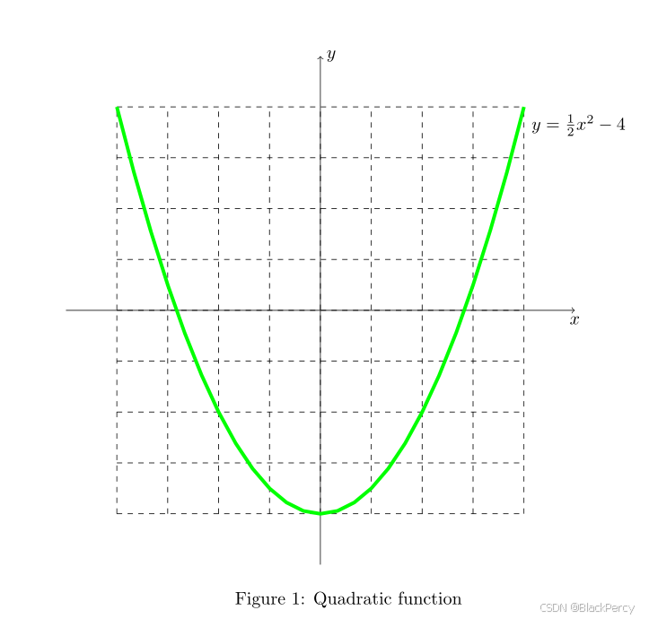
\draw[green,line width=2](-4,4)[domain=-4:4] plot({\x},{\x*\x/2-4})--(4,4)node[below right, black]{$y=\frac{1}{2}x^2-4$}; % 绘制二次曲线,起点,定义域,函数解析式,终点
\end{tikzpicture}
\caption{Quadratic function}
\label{fig:1}
\end{figure}
Figure \ref{fig:1} draws the graph of $y=\frac{1}{2}x^2-4$.效果
直角坐标系参数方程
latex
\begin{figure}[!hbtp]
\centering
\begin{tikzpicture}
\draw[->](-5,0)--(5,0)node[below]{$x$}; % 横轴
\draw[->](0,-5)--(0,5)node[right]{$y$}; % 纵轴
\draw[dashed](-4,-4) grid (4,4); % 平面网格
\fill[green!60!blue,opacity=90](0,2)[domain=0:360] plot({cos(\x)*2},{sin(\x)})--(0,2)node[below right, black]{$(2\cos(t),\sin(t))$};   % 绘制椭圆填充,起点,定义域,函数解析式,终点
\end{tikzpicture}
\caption{Quadratic function}
\label{fig:1}
\end{figure}
Figure \ref{fig:1} draws the graph of
$\left\{
\begin{array}{l l} x=&2\cos(t) \\ y=&\sin(t)
\end{array}
\right.$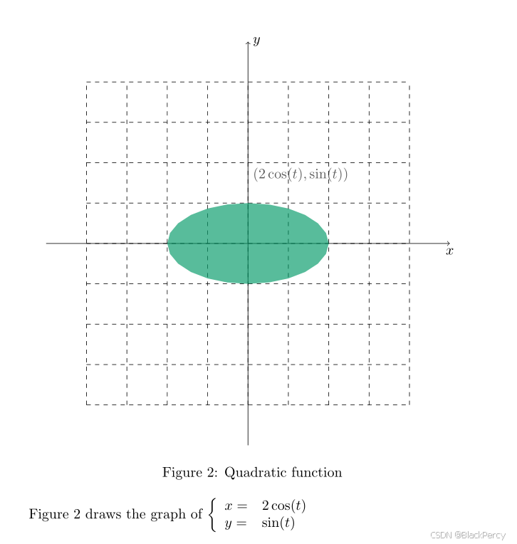
极坐标系
latex
\begin{figure}[!hbtp]
\centering
\begin{tikzpicture}
\foreach \r in {1,2,3} \draw[dashed] (0,0) circle (\r); % 同心圆
\foreach \a in {0,30,...,330} \draw[dashed] (0,0) -- (\a:3); % 放射线
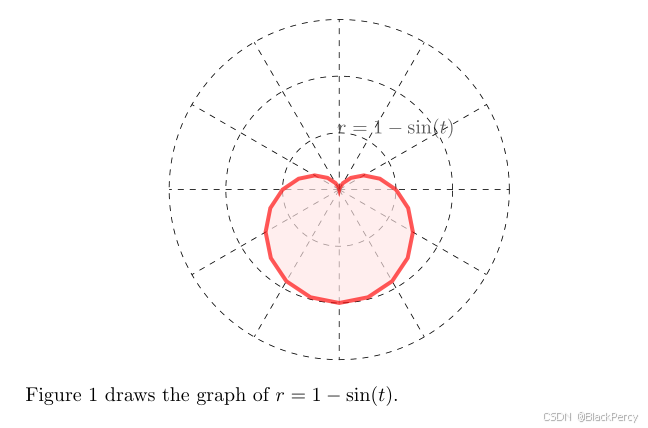
\filldraw[draw=red,fill=red!10,opacity=90,line width=2](0:1)[domain=0:360] plot({\x}:{1-sin(\x)})--(360:1)node[below=-40,]{$r=1-\sin(t)$}; % 绘制二次心形线的曲线与填充,起点,
\end{tikzpicture}
\end{figure}
Figure \ref{fig:1} draws the graph of $r=1-\sin(t)$.效果
韦恩图
latex
\begin{figure}[!hbtp]
\centering
\begin{tikzpicture}
    % 定义三个圆
    \def\circleA{(0,0) circle (1.5cm)}
    \def\circleB{(2,0) circle (1.5cm)}
    \def\circleC{(1,1.5) circle (1.5cm)}

    % 填充三个圆的公共交集(中心区域)
    \begin{scope}
        \clip \circleA;
        \clip \circleB;
        \fill[red!30] \circleC; % 红色半透明
    \end{scope}

    % 填充两两交集区域(示例:A和B的交集)
    \begin{scope}
        \clip \circleA;
        \fill[blue!20] \circleB; % 先填充A和B的交集
        \fill[white] \circleC;   % 然后用白色"挖掉"C覆盖的部分
    \end{scope}

    % 绘制圆的边框和标签
    \draw[thick] \circleA node[left] {$A$};
    \draw[thick] \circleB node[right] {$B$};
    \draw[thick] \circleC node[above] {$C$};

    % 可选:为不同区域添加文本标签
    \node at (1,- 2.5) {$A \cap B \cap \complement_{\Omega} C$};
\end{tikzpicture}
\end{figure}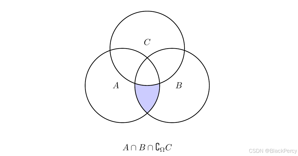
完整代码
latex
\documentclass{article}
\usepackage{tikz}

\begin{document}


\begin{figure}[!hbtp]
\centering
\begin{tikzpicture}
\draw[->](-5,0)--(5,0)node[below]{$x$}; % 横轴
\draw[->](0,-5)--(0,5)node[right]{$y$}; % 纵轴
\draw[dashed](-4,-4) grid (4,4); % 平面网格
\draw[green,line width=2](-4,4)[domain=-4:4] plot({\x},{\x*\x/2-4})--(4,4)node[below right, black]{$y=\frac{1}{2}x^2-4$};   % 绘制二次曲线,起点,定义域,函数解析式,终点
\end{tikzpicture}
\caption{Quadratic function}
\label{fig:1}
\end{figure}
Figure \ref{fig:1} draws the graph of $y=\frac{1}{2}x^2-4$.

\newpage
\begin{figure}[!hbtp]
\centering
\begin{tikzpicture}
\draw[->](-5,0)--(5,0)node[below]{$x$}; % 横轴
\draw[->](0,-5)--(0,5)node[right]{$y$}; % 纵轴
\draw[dashed](-4,-4) grid (4,4); % 平面网格
\fill[green!60!blue,opacity=90](0,2)[domain=0:360] plot({cos(\x)*2},{sin(\x)})--(0,2)node[below right, black]{$(2\cos(t),\sin(t))$};   % 绘制二次曲线,起点,定义域,函数解析式,终点
\end{tikzpicture}
\caption{Quadratic function}
\label{fig:1}
\end{figure}
Figure \ref{fig:1} draws the graph of
$\left\{
\begin{array}{l l} x=&2\cos(t) \\ y=&\sin(t)
\end{array}
\right.$

\newpage
\begin{figure}[!hbtp]
\centering
\begin{tikzpicture}
\foreach \r in {1,2,3} \draw[dashed] (0,0) circle (\r); % 同心圆
\foreach \a in {0,30,...,330} \draw[dashed] (0,0) -- (\a:3); % 放射线
\filldraw[draw=red,fill=red!10,opacity=90,line width=2](0:1)[domain=0:360] plot({\x}:{1-sin(\x)})--(360:1)node[below=-40,]{$r=1-\sin(t)$};   % 绘制二次曲线,起点,
\end{tikzpicture}
\end{figure}
Figure \ref{fig:1} draws the graph of $r=1-\sin(t)$.


\begin{figure}[!hbtp]
\centering
\begin{tikzpicture}
    % 定义三个圆
    \def\circleA{(0,0) circle (1.5cm)}
    \def\circleB{(2,0) circle (1.5cm)}
    \def\circleC{(1,1.5) circle (1.5cm)}

    % 填充三个圆的公共交集(中心区域)
    \begin{scope}
        \clip \circleA;
        \clip \circleB;
        \fill[red!30] \circleC; % 红色半透明
    \end{scope}

    % 填充两两交集区域(示例:A和B的交集)
    \begin{scope}
        \clip \circleA;
        \fill[blue!20] \circleB; % 先填充A和B的交集
        \fill[white] \circleC;   % 然后用白色"挖掉"C覆盖的部分
    \end{scope}

    % 绘制圆的边框和标签
    \draw[thick] \circleA node[left] {$A$};
    \draw[thick] \circleB node[right] {$B$};
    \draw[thick] \circleC node[above] {$C$};

    % 可选:为不同区域添加文本标签
    \node at (1,- 2.5) {$A \cap B \cap \complement_{\Omega} C$};
\end{tikzpicture}
\end{figure}
\end{document}