ResNet18 迁移学习实战：CIFAR-10 图像分类与 CPU 优化

引言

深度学习的发展历程中，网络深度一直是提升模型性能的关键因素。然而，传统深层网络面临着梯度消失 / 爆炸 和退化问题 ，限制了网络深度的进一步增加。2016 年，何恺明团队提出的ResNet（残差网络）通过引入残差连接，成功解决了深层网络的训练难题，在 ImageNet 比赛中取得了突破性成果。

一、ResNet 理论基础

1. 深层网络的挑战

传统 CNN 在加深网络深度时，会遇到两个主要问题：

梯度消失 / 爆炸：反向传播时，梯度经过多层网络后逐渐衰减或放大，导致底层网络难以训练
退化问题：当网络深度超过一定阈值后，模型性能开始下降，并非过拟合导致

2. 残差连接的创新

ResNet 通过引入残差块（Residual Block） ，解决了深层网络的训练难题。残差块的核心思想是：让网络学习残差映射，而非直接学习恒等映射。

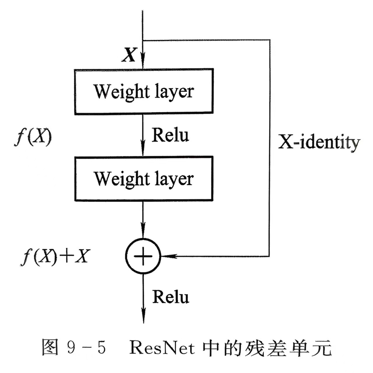
数学原理

对于一个深层网络，假设期望的底层映射为H(x)，ResNet 将其分解为：H(x) = F(x) + x

其中：

x：输入特征
F(x)：残差映射（网络需要学习的部分）
F(x) + x：恒等映射（通过 shortcut 连接直接传递）

优势分析

缓解梯度消失：残差连接提供了梯度直接传播的路径，底层网络能够获得有效的梯度更新
易于优化：学习残差映射F(x)比直接学习H(x)更容易，尤其是当H(x)接近恒等映射时
支持更深网络：ResNet 成功训练了 152 层甚至更深的网络，突破了传统 CNN 的深度限制

3. ResNet18 网络结构

ResNet18 包含18 层可训练层（16 个卷积层 + 2 个全连接层），由 8 个残差块组成：

模块	残差块数量	输出通道	步长	输出尺寸
Conv1	-	64	2	112×112
MaxPool	-	64	2	56×56
Layer1	2	64	1	56×56
Layer2	2	128	2	28×28
Layer3	2	256	2	14×14
Layer4	2	512	2	7×7
AvgPool	-	512	-	1×1
FC	-	1000	-	-

二、实验配置

核心配置参数

python 复制代码

DEVICE = torch.device("cuda" if torch.cuda.is_available() else "cpu")
BATCH_SIZE = 32  # CPU优化：平衡内存与速度
EPOCHS = 10       # 快速收敛
LEARNING_RATE = 5e-4  # 适合迁移学习的学习率
NUM_CLASSES = 10  # CIFAR-10类别数

三、代码实现与优化

1. 数据预处理与增强

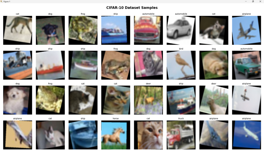
针对 CIFAR-10 数据集（32×32 彩色图像），设计了高效的数据预处理流程：

python 复制代码

cifar_mean = [0.4914, 0.4822, 0.4465]
cifar_std = [0.2023, 0.1994, 0.2010]

transform_train = transforms.Compose([
    transforms.RandomCrop(32, padding=4),  # 随机裁剪，增强泛化能力
    transforms.Resize((224, 224)),  # 调整为ResNet输入尺寸
    transforms.RandomHorizontalFlip(p=0.5),  # 随机水平翻转
    transforms.RandomRotation(15),  # 随机旋转±15°
    transforms.ToTensor(),
    transforms.Normalize(mean=cifar_mean, std=cifar_std)  # CIFAR-10专用归一化
])

优化点解析：

使用CIFAR-10 专用归一化参数：相比 ImageNet 参数，更适合目标数据集
增加多种数据增强：随机裁剪、翻转、旋转，有效减少过拟合
调整为224×224 输入尺寸：适配 ResNet 预训练模型的输入要求

2. 数据加载优化

针对 CPU 环境，对数据加载进行了优化：

python 复制代码

train_loader = DataLoader(
    train_dataset, batch_size=BATCH_SIZE, shuffle=True,
    num_workers=0, pin_memory=False  # CPU优化：禁用多线程+锁存
)

优化点解析：

num_workers=0：CPU 环境下禁用多线程，避免线程切换开销
pin_memory=False：CPU 环境下禁用内存锁存，减少内存占用
BATCH_SIZE=32：平衡内存占用与训练速度，避免 CPU 内存溢出

3. ResNet18 模型构建与微调

python 复制代码

model = models.resnet18(weights=ResNet18_Weights.IMAGENET1K_V1)

# 迁移学习策略：冻结底层，解冻顶层卷积块+全连接层
for param in model.parameters():
    param.requires_grad = False  # 冻结所有层
for param in model.layer4.parameters():
    param.requires_grad = True  # 解冻最后一个卷积块（layer4）

# 替换全连接层，适配10分类任务
in_features = model.fc.in_features
model.fc = nn.Sequential(
    nn.Dropout(0.5),  # 添加Dropout，防止过拟合
    nn.Linear(in_features, NUM_CLASSES)
)
model = model.to(DEVICE)

优化点解析：

加载预训练权重：使用 ImageNet 预训练权重，加速模型收敛
分层冻结策略：仅解冻顶层卷积块（layer4），兼顾特征微调与训练速度
添加 Dropout：在全连接层前添加 Dropout (0.5)，有效防止过拟合
替换分类层：将输出类别数从 1000 改为 10，适配 CIFAR-10 任务

4. 优化器与学习率调度

python 复制代码

# 使用AdamW优化器，结合权重衰减，适合深度学习训练
optimizer = optim.AdamW(
    filter(lambda p: p.requires_grad, model.parameters()),  # 仅优化可训练参数
    lr=LEARNING_RATE, weight_decay=1e-4  # 权重衰减抑制过拟合
)

# 动态学习率调度：当准确率不再提升时，自动降低学习率
scheduler = optim.lr_scheduler.ReduceLROnPlateau(
    optimizer, mode='max', patience=2, factor=0.5
)

优化点解析：

AdamW 优化器：相比传统 Adam，结合了权重衰减，更适合深层网络训练
动态学习率：使用 ReduceLROnPlateau，当验证准确率停滞时自动将学习率减半
仅优化可训练参数：使用 filter 函数，减少不必要的计算开销

5. 训练函数优化

python 复制代码

def train_model(model, train_loader, test_loader, criterion, optimizer, scheduler, epochs):
    train_losses = []
    test_accuracies = []
    best_acc = 0.0

    for epoch in range(epochs):
        start_time = time.time()

        # 训练阶段
        model.train()
        running_loss = 0.0
        for batch_idx, (data, targets) in enumerate(train_loader):
            data, targets = data.to(DEVICE), targets.to(DEVICE)

            outputs = model(data)
            loss = criterion(outputs, targets)

            optimizer.zero_grad()
            loss.backward()
            optimizer.step()

            running_loss += loss.item() * data.size(0)

            # CPU优化：降低打印频率
            if batch_idx % 200 == 0 and batch_idx != 0:
                print(f'  Batch {batch_idx}/{len(train_loader)}, Loss: {loss.item():.4f}')

        # 验证阶段（精简代码，减少冗余计算）
        model.eval()
        test_correct = 0
        with torch.no_grad():
            for data, targets in test_loader:
                data, targets = data.to(DEVICE), targets.to(DEVICE)
                outputs = model(data)
                _, predicted = torch.max(outputs, 1)
                test_correct += (predicted == targets).sum().item()

        test_acc = 100 * test_correct / len(test_loader.dataset)
        test_accuracies.append(test_acc)

        # 学习率调度
        scheduler.step(test_acc)

        # 保存最佳模型
        if test_acc > best_acc:
            best_acc = test_acc
            torch.save(model.state_dict(), "best_resnet_cifar10.pth")

        print(f'Epoch [{epoch+1}/{epochs}] | Loss: {epoch_loss:.4f} | Test Acc: {test_acc:.2f}% | Time: {epoch_time:.1f}s')

    return train_losses, test_accuracies

优化点解析：

降低打印频率：每 200 批次打印一次，减少 CPU IO 开销
精简验证代码：去除冗余计算，提高验证速度
仅保存最佳模型：避免频繁写入磁盘，减少 IO 操作
记录核心指标：仅记录训练损失和测试准确率，简化日志

四、实验结果与分析

1. 数据集样本展示

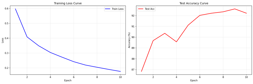
2. 训练曲线

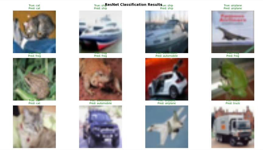
3. 分类结果展示

4. ResNet18 优势分析

残差连接：有效解决了深层网络的梯度消失问题，训练 18 层网络依然稳定
轻量级设计：ResNet18 参数量相比 VGG16 轻量得多，适合 CPU 环境
泛化能力强：预训练模型在 ImageNet 上学到的特征具有很强的通用性，迁移到 CIFAR-10 效果显著
易于微调：分层冻结策略使得模型在小数据集上易于微调，快速适应新任务

五、完整代码

python 复制代码

import torch
import torch.nn as nn
import torch.optim as optim
from torchvision import datasets, transforms, models
from torchvision.models import ResNet18_Weights
from torch.utils.data import DataLoader
import time
import matplotlib.pyplot as plt
import numpy as np
from PIL import Image

# ---------------------- 1. 核心配置----------------------
DEVICE = torch.device("cuda" if torch.cuda.is_available() else "cpu")

# CPU环境优化配置
BATCH_SIZE = 32  # CPU批次不宜过大
EPOCHS = 10
LEARNING_RATE = 5e-4
NUM_CLASSES = 10
classes = ['airplane', 'automobile', 'bird', 'cat', 'deer',
           'dog', 'frog', 'horse', 'ship', 'truck']

# ---------------------- 2. 优化数据预处理 ----------------------
cifar_mean = [0.4914, 0.4822, 0.4465]
cifar_std = [0.2023, 0.1994, 0.2010]

transform_train = transforms.Compose([
    transforms.RandomCrop(32, padding=4),
    transforms.Resize((224, 224)),
    transforms.RandomHorizontalFlip(p=0.5),
    transforms.RandomRotation(15),
    transforms.ToTensor(),
    transforms.Normalize(mean=cifar_mean, std=cifar_std)
])

transform_test = transforms.Compose([
    transforms.Resize((224, 224)),
    transforms.ToTensor(),
    transforms.Normalize(mean=cifar_mean, std=cifar_std)
])

# ---------------------- 3. 数据加载 ----------------------
train_dataset = datasets.CIFAR10(root='./data', train=True, download=True, transform=transform_train)
test_dataset = datasets.CIFAR10(root='./data', train=False, download=True, transform=transform_test)

# CPU环境：num_workers=0 + pin_memory=False
train_loader = DataLoader(
    train_dataset, batch_size=BATCH_SIZE, shuffle=True,
    num_workers=0, pin_memory=False
)
test_loader = DataLoader(
    test_dataset, batch_size=BATCH_SIZE, shuffle=False,
    num_workers=0, pin_memory=False
)


# ---------------------- 4. 数据集展示 ----------------------
def show_dataset_samples():
    data_iter = iter(train_loader)
    images, labels = next(data_iter)

    fig, axes = plt.subplots(4, 8, figsize=(16, 8))
    fig.suptitle('CIFAR-10 Dataset Samples', fontsize=16, fontweight='bold')

    for i in range(32):
        row, col = i // 8, i % 8
        img = images[i].numpy().transpose((1, 2, 0))
        img = img * cifar_std + cifar_mean
        img = np.clip(img, 0, 1)

        axes[row, col].imshow(img)
        axes[row, col].set_title(classes[labels[i]], fontsize=10)
        axes[row, col].axis('off')

    plt.tight_layout()
    plt.savefig('dataset_samples.png', dpi=150, bbox_inches='tight')
    plt.show()


print("展示数据集样本...")
show_dataset_samples()

# ---------------------- 5. 模型优化 ----------------------
model = models.resnet18(weights=ResNet18_Weights.IMAGENET1K_V1)

# 冻结底层，解冻顶层卷积块+全连接层
for param in model.parameters():
    param.requires_grad = False
for param in model.layer4.parameters():
    param.requires_grad = True

# 替换全连接层
in_features = model.fc.in_features
model.fc = nn.Sequential(
    nn.Dropout(0.5),
    nn.Linear(in_features, NUM_CLASSES)
)
model = model.to(DEVICE)

# ---------------------- 6. 优化器 ----------------------
criterion = nn.CrossEntropyLoss()
optimizer = optim.AdamW(
    filter(lambda p: p.requires_grad, model.parameters()),
    lr=LEARNING_RATE, weight_decay=1e-4
)

scheduler = optim.lr_scheduler.ReduceLROnPlateau(
    optimizer, mode='max', patience=2, factor=0.5
)


# ---------------------- 7. 训练函数 ----------------------
def train_model(model, train_loader, test_loader, criterion, optimizer, scheduler, epochs):
    train_losses = []
    test_accuracies = []
    best_acc = 0.0

    for epoch in range(epochs):
        start_time = time.time()

        # 训练阶段
        model.train()
        running_loss = 0.0
        for batch_idx, (data, targets) in enumerate(train_loader):
            data, targets = data.to(DEVICE), targets.to(DEVICE)

            outputs = model(data)
            loss = criterion(outputs, targets)

            optimizer.zero_grad()
            loss.backward()
            optimizer.step()

            running_loss += loss.item() * data.size(0)

            # CPU训练打印频率降低
            if batch_idx % 200 == 0 and batch_idx != 0:
                print(f'  Batch {batch_idx}/{len(train_loader)}, Loss: {loss.item():.4f}')

        epoch_loss = running_loss / len(train_loader.dataset)
        train_losses.append(epoch_loss)

        # 验证阶段
        model.eval()
        test_correct = 0
        with torch.no_grad():
            for data, targets in test_loader:
                data, targets = data.to(DEVICE), targets.to(DEVICE)
                outputs = model(data)
                _, predicted = torch.max(outputs, 1)
                test_correct += (predicted == targets).sum().item()

        test_acc = 100 * test_correct / len(test_loader.dataset)
        test_accuracies.append(test_acc)
        epoch_time = time.time() - start_time

        # 学习率调度
        scheduler.step(test_acc)

        print(
            f'Epoch [{epoch + 1}/{epochs}] | Loss: {epoch_loss:.4f} | Test Acc: {test_acc:.2f}% | Time: {epoch_time:.1f}s')

        # 保存最佳模型
        if test_acc > best_acc:
            best_acc = test_acc
            torch.save(model.state_dict(), "best_resnet_cifar10.pth")
            print(f'  Best model saved! Acc: {best_acc:.2f}%')

    return train_losses, test_accuracies


# ---------------------- 8. 训练曲线 ----------------------
def plot_training_curves(train_losses, test_accuracies):
    fig, (ax1, ax2) = plt.subplots(1, 2, figsize=(15, 5))

    ax1.plot(range(1, EPOCHS + 1), train_losses, 'b-', linewidth=2, label='Train Loss')
    ax1.set_xlabel('Epoch')
    ax1.set_ylabel('Loss')
    ax1.set_title('Training Loss Curve')
    ax1.grid(True, alpha=0.3)
    ax1.legend()

    ax2.plot(range(1, EPOCHS + 1), test_accuracies, 'r-', linewidth=2, label='Test Acc')
    ax2.set_xlabel('Epoch')
    ax2.set_ylabel('Accuracy (%)')
    ax2.set_title('Test Accuracy Curve')
    ax2.grid(True, alpha=0.3)
    ax2.legend()

    plt.tight_layout()
    plt.savefig('training_curves.png', dpi=150, bbox_inches='tight')
    plt.show()


# ---------------------- 9. 分类结果展示 ----------------------
def show_classification_results(model, test_loader):
    model.eval()
    images, labels = next(iter(test_loader))
    images = images.to(DEVICE)

    with torch.no_grad():
        outputs = model(images)
        _, predictions = torch.max(outputs, 1)

    fig, axes = plt.subplots(3, 4, figsize=(15, 12))
    fig.suptitle('ResNet Classification Results', fontsize=16, fontweight='bold')

    for i in range(12):
        row, col = i // 4, i % 4
        img = images[i].cpu().numpy().transpose((1, 2, 0))
        img = img * cifar_std + cifar_mean
        img = np.clip(img, 0, 1)

        axes[row, col].imshow(img)
        true_label = classes[labels[i]]
        pred_label = classes[predictions[i]]
        color = 'green' if true_label == pred_label else 'red'
        axes[row, col].set_title(f'True: {true_label}\nPred: {pred_label}', color=color, fontsize=12)
        axes[row, col].axis('off')

    plt.tight_layout()
    plt.savefig('classification_results.png', dpi=150, bbox_inches='tight')
    plt.show()

    acc = 100 * (predictions.cpu() == labels).sum().item() / len(labels)
    print(f'示例批次准确率: {acc:.2f}%')


# ---------------------- 10. 主训练流程 ----------------------
if __name__ == "__main__":
    print("=" * 60)
    print(f"开始训练 | Epochs={EPOCHS}, Batch={BATCH_SIZE}, LR={LEARNING_RATE}")
    print("=" * 60)

    train_losses, test_accuracies = train_model(
        model, train_loader, test_loader, criterion, optimizer, scheduler, EPOCHS
    )

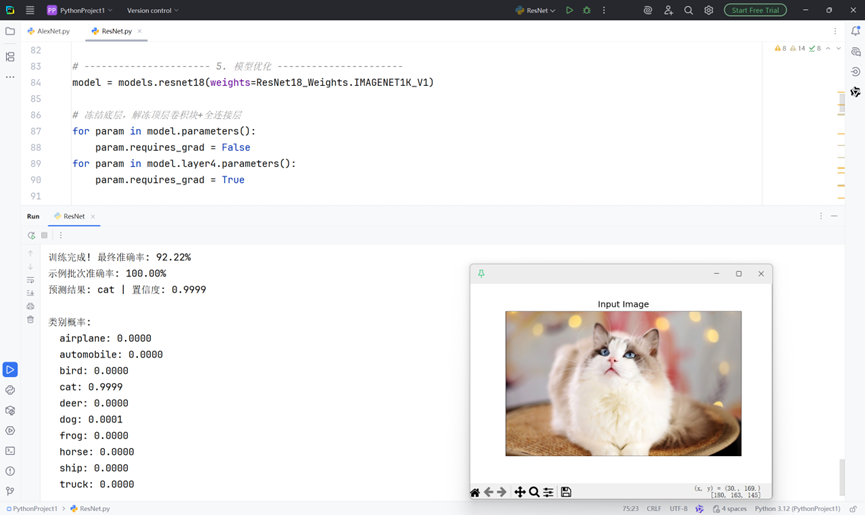
    print(f"\n训练完成! 最终准确率: {test_accuracies[-1]:.2f}%")

    # 核心展示
    plot_training_curves(train_losses, test_accuracies)
    show_classification_results(model, test_loader)

# ---------------------- 11. 单张图像预测 ----------------------
def predict_single_image(image_path="test_image.jpg"):
    # 加载模型
    model = models.resnet18(weights=None)
    in_features = model.fc.in_features
    model.fc = nn.Sequential(nn.Dropout(0.5), nn.Linear(in_features, NUM_CLASSES))
    model.load_state_dict(torch.load("best_resnet_cifar10.pth", map_location=DEVICE))
    model.to(DEVICE).eval()

    # 预处理
    transform = transforms.Compose([
        transforms.Resize((224, 224)),
        transforms.ToTensor(),
        transforms.Normalize(mean=cifar_mean, std=cifar_std)
    ])

    # 加载显示图像
    try:
        image = Image.open(image_path).convert("RGB")
        plt.figure(figsize=(6, 6)), plt.imshow(image), plt.axis('off'), plt.title("Input Image"), plt.show()

        # 预测
        with torch.no_grad():
            img_tensor = transform(image).unsqueeze(0).to(DEVICE)
            outputs = model(img_tensor)
            probs = torch.softmax(outputs, dim=1)
            conf, pred = torch.max(probs, 1)

        print(f"预测结果: {classes[pred.item()]} | 置信度: {conf.item():.4f}")
        print("\n类别概率:")
        for cls, p in zip(classes, probs.cpu().numpy()[0]):
            print(f"  {cls}: {p:.4f}")
    except FileNotFoundError:
        print(f"错误：未找到图像文件 {image_path}，请确保文件存在")

# 示例调用
predict_single_image("test_image.jpg")