单细胞转录组分析流程十一（细胞通讯，cellchat，双（多）样本）

前言

在上一期中，我们已经完整讲解了 CellChat 在单样本中的使用流程 ，从数据准备、信号通路推断，到可视化展示细胞之间的交流方式。然而，在真实的生物医学研究中，最常见、最有价值的情境并不是单个样本 ，而是 ------
比较两类不同的生物状态在细胞通讯上的差异。

无论是 疾病组 vs 正常组、治疗前 vs 治疗后、野生型 vs 突变型、肿瘤中心 vs 边缘 ，研究者最关心的往往都是：

哪些细胞的通讯增强了？

哪些信号通路被抑制了？

哪些细胞间的互动发生了重塑？

双样本 CellChat 分析正是为了解决这些问题。

通过构建两个 CellChat 对象，并进行合并、对比、差异分析，研究者可以系统性地揭示细胞通讯网络在不同状态下的变化模式，从而更深入理解微环境调控、疾病发生机制以及治疗干预效果。

这一篇专栏将带你系统掌握 双样本 CellChat 分析的完整流程 ------ 是实际科研中最常用、最具解释力的分析方式。

一、数据准备

CellChat 的输入数据结构非常固定，只需要两个核心数据**，细胞表达矩阵（标准化之后）** 和细胞 metadata（带有 cell type 信息）

注意：双样本 CellChat 对比分析强烈建议保持两个样本的细胞注释一致，且每类细胞只能数量最好大于10！！！

如果两个数据集细胞注释不一致，可以使用，多个不同细胞组成的细胞集

由于前期注释是在大群注释，如果注释太过精细，那么在分散到每个样本中的细胞可能很少，因此使用T细胞群的中等分群进行分析

R 复制代码

library(Seurat)
library(CellChat)

# 读取之前的数据
scRNA <- readRDS("D:/datat/新建文件夹/GSE191288_RAW/scRNA.rds")
T_sce <- readRDS("D:/datat/新建文件夹/GSE191288_RAW/T_sce.rds")
B_sce <- readRDS("D:/datat/新建文件夹/GSE191288_RAW/B_sce.rds")

# 子集注释回写母对象
phe <- scRNA@meta.data
phe_T <- T_sce@meta.data

# 如有因子，先转换为字符
phe$celltype <- as.character(phe$celltype)
phe_T$celltype.1 <- as.character(phe_T$celltype.1)

# 找到匹配的行
common_T <- intersect(rownames(phe), rownames(phe_T))

# 回写细胞类型
phe[common_T, "celltype"] <- phe_T[common_T, "celltype.1"]

scRNA@meta.data <- phe

table(phe$orig.ident,phe$celltype)
     
# B Cells CD 4 CD 8 Endothelial Epithelial Cells Fibroblasts Cells Myeloid Cells   NK  NKT γδ T
# NT       12   55   79        1122              909               878            51   58    1   28
# T1L      60  139  111         663              135              1390            67   25    4   30
# T1R     300  637  363         222               66               425           192   22   16   82
# T2L      48  834  570         191              164               406           150  261   20  191
# T2R     559 1005  398         191               31               166           114  100   11   67
# T3L      11  260  160          60             1506               336           269   40   13   29
# T3R       5  175  332         159             3113               188           164   62    6   54

## NT为癌旁组织，其余为甲状腺组织（临床分型为PTC）
## 本次流程使用癌旁组织（NT）和 甲状腺组织（T1L）

发现对于NKT细胞群，NT样本只有1个，T1L只有4个NKT，明显不符合分析标准，可以选择删除（subset）或将其归类于上类细胞群（也就是把NKT归类于NK细胞）

使用SplitObject()拆分多样本

拆出的结果：obj.list 是一个 list；每个元素都是一个独立的 Seurat 对象

R 复制代码

obj.list <- SplitObject(scRNA, split.by = "orig.ident")
print(obj.list)
$T1L
An object of class Seurat 
28858 features across 2624 samples within 1 assay 
Active assay: RNA (28858 features, 2000 variable features)
 3 layers present: data, counts, scale.data
 4 dimensional reductions calculated: pca, harmony, umap, tsne

$T1R
An object of class Seurat 
28858 features across 2325 samples within 1 assay 
Active assay: RNA (28858 features, 2000 variable features)
 3 layers present: data, counts, scale.data
 4 dimensional reductions calculated: pca, harmony, umap, tsne

$T2L
An object of class Seurat 
28858 features across 2835 samples within 1 assay 
Active assay: RNA (28858 features, 2000 variable features)
 3 layers present: data, counts, scale.data
 4 dimensional reductions calculated: pca, harmony, umap, tsne

$T2R
An object of class Seurat 
28858 features across 2642 samples within 1 assay 
Active assay: RNA (28858 features, 2000 variable features)
 3 layers present: data, counts, scale.data
 4 dimensional reductions calculated: pca, harmony, umap, tsne

$T3L
An object of class Seurat 
28858 features across 2684 samples within 1 assay 
Active assay: RNA (28858 features, 2000 variable features)
 3 layers present: data, counts, scale.data
 4 dimensional reductions calculated: pca, harmony, umap, tsne

$T3R
An object of class Seurat 
28858 features across 4258 samples within 1 assay 
Active assay: RNA (28858 features, 2000 variable features)
 3 layers present: data, counts, scale.data
 4 dimensional reductions calculated: pca, harmony, umap, tsne

$NT
An object of class Seurat 
28858 features across 3193 samples within 1 assay 
Active assay: RNA (28858 features, 2000 variable features)
 3 layers present: data, counts, scale.data
 4 dimensional reductions calculated: pca, harmony, umap, tsne

分别提取两个样本数据（使用NT和T1L）

R 复制代码

obj.list[["NT"]] <- subset(obj.list[["NT"]], subset = celltype != "NKT")
obj.list[["T1L"]] <- subset(obj.list[["T1L"]], subset = celltype != "NKT")
table(obj.list[["NT"]]$celltype)
#          B Cells              CD 4              CD 8       Endothelial  Epithelial Cells Fibroblasts Cells     Myeloid Cells 
#              12                55                79              1122               909               878                51 
#              NK              γδ T 
#              58                28 
table(obj.list[["T1L"]]$celltype)
#          B Cells              CD 4              CD 8       Endothelial  Epithelial Cells Fibroblasts Cells     Myeloid Cells 
#              60               139               111               663               135              1390                67 
#              NK              γδ T 
#              25                30 


 
# 根据研究情况进行细胞排序
celltype_order <- c(
  "CD 4", 
  "CD 8", 
  "γδ T", 
  "NK", 
  "B Cells", 
  "Myeloid Cells", 
  "Fibroblasts Cells", 
  "Epithelial Cells", 
  "Endothelial"
)
 

# 如果样本多可以写一个循环

## 细胞的基因表达数据，由于每个样本只删除几个细胞，所以不需要再做标准化，直接提取就可以
data.input_NT <- GetAssayData(obj.list[["NT"]], slot = 'data') # normalized data matrix
data.input_T1L <- GetAssayData(obj.list[["T1L"]], slot = 'data') # normalized data matrix
## metadata文件
meta_NT <- obj.list[["NT"]]@meta.data[,c("orig.ident","celltype")]
meta_T1L <- obj.list[["T1L"]]@meta.data[,c("orig.ident","celltype")]

# 对 meta 和 data.input 进行排序（NT样本）
identical(rownames(meta_NT), colnames(data.input_NT))
meta_NT$celltype <- factor(meta_NT$celltype ,levels = celltype_order)
ordered_indices <- order(meta_NT$celltype)
 
meta_NT <- meta_NT[ordered_indices, ]
data.input_NT <- data.input_NT[, ordered_indices]
identical(rownames(meta_NT),colnames(data.input_NT))

# 对 meta 和 data.input 进行排序（T1L样本）
identical(rownames(meta_T1L), colnames(data.input_T1L))
meta_T1L$celltype <- factor(meta_T1L$celltype ,levels = celltype_order)
ordered_indices <- order(meta_T1L$celltype)
 
meta_T1L <- meta_T1L[ordered_indices, ]
data.input_T1L <- data.input_T1L[, ordered_indices]
identical(rownames(meta_T1L),colnames(data.input_T1L))

创建cellchat对象

R 复制代码

# 加载数据库
CellChatDB <- CellChatDB.human  #人源样本
# 查看数据的分类情况与
# 具体内容showDatabaseCategory(CellChatDB)
dplyr::glimpse(CellChatDB$interaction)
 
#筛选数据库，只保留"Secreted Signaling"
CellChatDB.use <- subsetDB(CellChatDB, search = "Secreted Signaling")
 
## NT样品
cellchat_NT <- createCellChat(object = data.input_NT, meta = meta_NT, group.by = "celltype")
# 添加细胞信息
cellchat_NT <- addMeta(cellchat_NT, meta = meta_NT)
cellchat_NT <- setIdent(cellchat_NT, ident.use = "celltype") 
levels(cellchat_NT@idents) 
groupSize_NT <- as.numeric(table(cellchat_NT@idents))

cellchat_NT@DB <- CellChatDB.use
cellchat_NT <- subsetData(cellchat_NT) # 只保留 配体/受体基因的表达矩阵
# 类似于找高变基因
cellchat_NT <- identifyOverExpressedGenes(cellchat_NT)
cellchat_NT <- identifyOverExpressedInteractions(cellchat_NT)
cellchat_NT <- computeCommunProb(cellchat_NT, type = "triMean")
cellchat_NT <- filterCommunication(cellchat_NT, min.cells = 10)
cellchat_NT <- computeCommunProbPathway(cellchat_NT)
cellchat_NT <- aggregateNet(cellchat_NT)
cellchat_NT <- netAnalysis_computeCentrality(cellchat_NT, slot.name = "netP") 


## T1L样品
cellchat_T1L <- createCellChat(object = data.input_T1L, meta = meta_T1L, group.by = "celltype")
# 添加细胞信息
cellchat_T1L <- addMeta(cellchat_T1L, meta = meta_T1L)
cellchat_T1L <- setIdent(cellchat_T1L, ident.use = "celltype") 
levels(cellchat_T1L@idents) 
groupSize_T1L <- as.numeric(table(cellchat_T1L@idents))

cellchat_T1L@DB <- CellChatDB.use
cellchat_T1L <- subsetData(cellchat_T1L) # 只保留 配体/受体基因的表达矩阵
# 类似于找高变基因
cellchat_T1L <- identifyOverExpressedGenes(cellchat_T1L)
cellchat_T1L <- identifyOverExpressedInteractions(cellchat_T1L)
cellchat_T1L <- computeCommunProb(cellchat_T1L, type = "triMean")
cellchat_T1L <- filterCommunication(cellchat_T1L, min.cells = 10)
cellchat_T1L <- computeCommunProbPathway(cellchat_T1L)
cellchat_T1L <- aggregateNet(cellchat_T1L)
cellchat_T1L <-netAnalysis_computeCentrality(cellchat_T1L, slot.name = "netP")

合并两样本

R 复制代码

object.list <- list(NT=cellchat_NT,T1L=cellchat_T1L)
cellchat <- mergeCellChat(object.list, add.names = names(object.list))
cellchat

比较相互作用的总数和互作强度

1.整体比较

R 复制代码

1.整体比较
gg1 <- compareInteractions(cellchat, show.legend = F, 
                           group = c(1,2))
gg2 <- compareInteractions(cellchat, show.legend = F, 
                           group = c(1,2),measure = "weight")
gg1 + gg2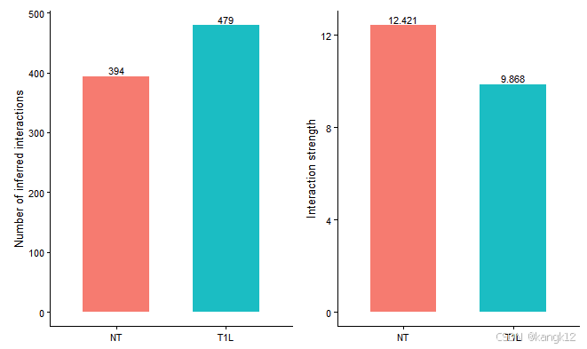

CellChat比较了从不同生物条件下推断出的细胞间通讯网络的相互作用总数和相互作用强度。在该数据集中，NT的互作数量小于T1L样本，但是NT样本的信号强度高于T1L样本

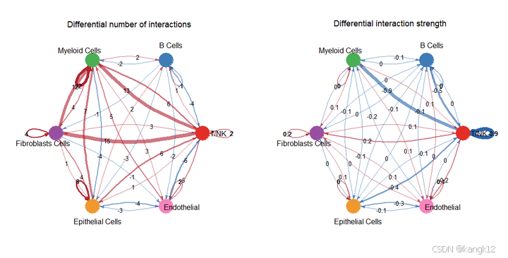
2.比较不同细胞群体之间的互作数量和强度

R 复制代码

netVisual_diffInteraction(cellchat, weight.scale = T)
netVisual_diffInteraction(cellchat, weight.scale = T, measure = "weight")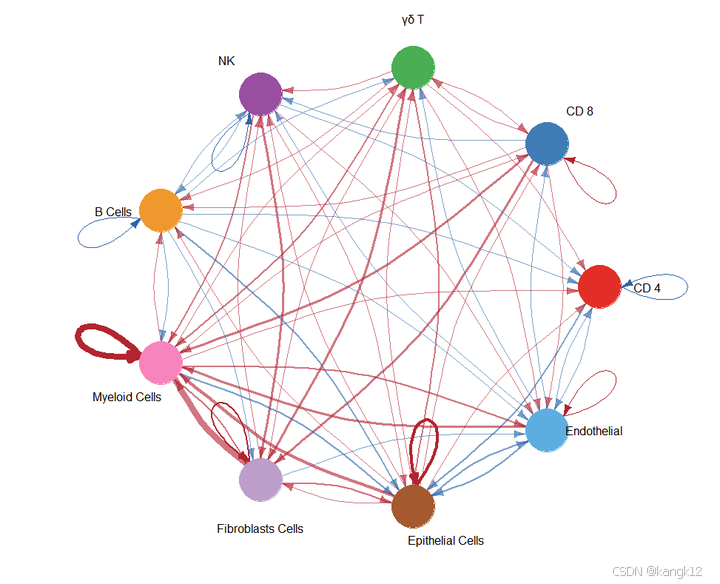

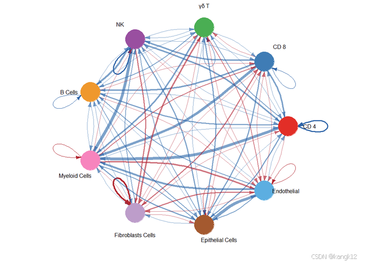
通过圆形可视化两个数据集中细胞间通讯网络中相互作用数量的差异或相互作用强度，其中红色或者蓝色的着色边代表与第一个数据集相比，第二个数据集中上调或者下调的信号。分组顺序是按照object.list中的顺序而定的。

3.显示两个数据集中不同细胞群体间相互作用数量或相互作用强度

热图

R 复制代码

gg1 <- netVisual_heatmap(cellchat)
gg2 <- netVisual_heatmap(cellchat, measure = "weight")

gg1 + gg2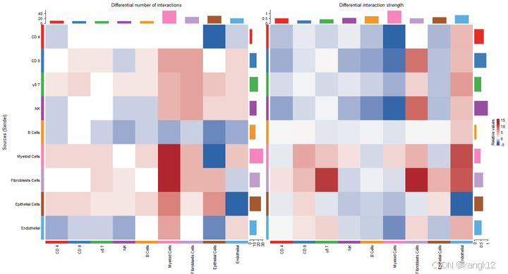

顶部彩色条形图表示热图中显示的每列绝对值之和（传入信号）。右侧彩色条形图表示每行绝对值之和（传出信号）。因此，条形高度表示两个条件之间交互数量或交互强度变化的程度。在颜色条中，红色或者蓝色表示与第一个数据集相比，第二个数据集中上调或者下调的信号。

Circe图

（和上面的热图二选一）

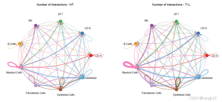
4.Circle图显示粗细胞类型之间的相互作用数量或相互作用强度差异

可以理解为对细胞群重新分组

R 复制代码

# 按照celltype_order进行分组
celltype_order
# 分组，把所有T细胞分为一组，如果是自己的数据集，可以按照研究目的进行分组
group.cellType <- c(rep("T/NK", 4), "B Cells", "Myeloid Cells", "Fibroblasts Cells",  "Epithelial Cells", "Endothelial")
group.cellType <- factor(group.cellType, levels = c("T/NK",  "B Cells", "Myeloid Cells", "Fibroblasts Cells",  "Epithelial Cells", "Endothelial"))
object.list <- lapply(object.list, function(x) {mergeInteractions(x, group.cellType)})
cellchat <- mergeCellChat(object.list, add.names = names(object.list))

weight.max <- getMaxWeight(object.list, slot.name = c("idents", "net", "net"), attribute = c("idents","count", "count.merged"))
# interactions
par(mfrow = c(1,2), xpd=TRUE)
for (i in 1:length(object.list)) {
  netVisual_circle(object.list[[i]]@net$count.merged, weight.scale = T, label.edge= T, edge.weight.max = weight.max[3], edge.width.max = 12, title.name = paste0("Number of interactions - ", names(object.list)[i]))
}

# weight.merged
par(mfrow = c(1,2), xpd=TRUE)
netVisual_diffInteraction(cellchat, weight.scale = T, measure = "count.merged", label.edge = T)
netVisual_diffInteraction(cellchat, weight.scale = T, measure = "weight.merged", label.edge = T)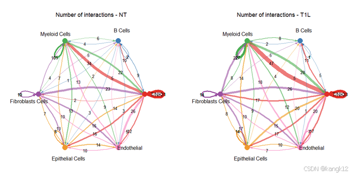

5.在二维空间中比较主要来源和目标

识别发送或接收信号发生显著变化的细胞群体

R 复制代码

num.link <- sapply(object.list, function(x) {rowSums(x@net$count) + colSums(x@net$count)-diag(x@net$count)})
weight.MinMax <- c(min(num.link), max(num.link)) # control the dot size in the different datasets
gg <- list()
for (i in 1:length(object.list)) {
  gg[[i]] <- netAnalysis_signalingRole_scatter(object.list[[i]], title = names(object.list)[i], weight.MinMax = weight.MinMax)
}

patchwork::wrap_plots(plots = gg)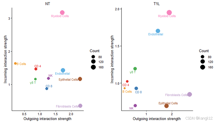

差异还是挺大的，毕竟是一个肿瘤一个癌旁

识别特定细胞群体的信号变化

R 复制代码

# 可视化从NT样本到T1L样本的发出与接收信号差异变化，指定细胞和通路
gg1 <- netAnalysis_signalingChanges_scatter(cellchat, idents.use = "Endothelial", signaling.exclude = "MIF")
gg2 <- netAnalysis_signalingChanges_scatter(cellchat, idents.use = "CD 4", signaling.exclude = c("MIF"))

patchwork::wrap_plots(plots = list(gg1,gg2))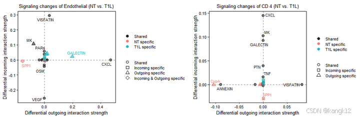

按照github中作者的解释，正值表示在第二种情况中升高，负值表示在第一种情况中升高。

6.识别具有不同相互作用强度的改变信号

比较每个信号通路或配体-受体对的总体信息流

R 复制代码

gg1 <- rankNet(cellchat, mode = "comparison", measure = "weight", sources.use = NULL, targets.use = NULL, stacked = T, do.stat = TRUE)
gg2 <- rankNet(cellchat, mode = "comparison", measure = "weight", sources.use = NULL, targets.use = NULL, stacked = F, do.stat = TRUE)

gg1 + gg2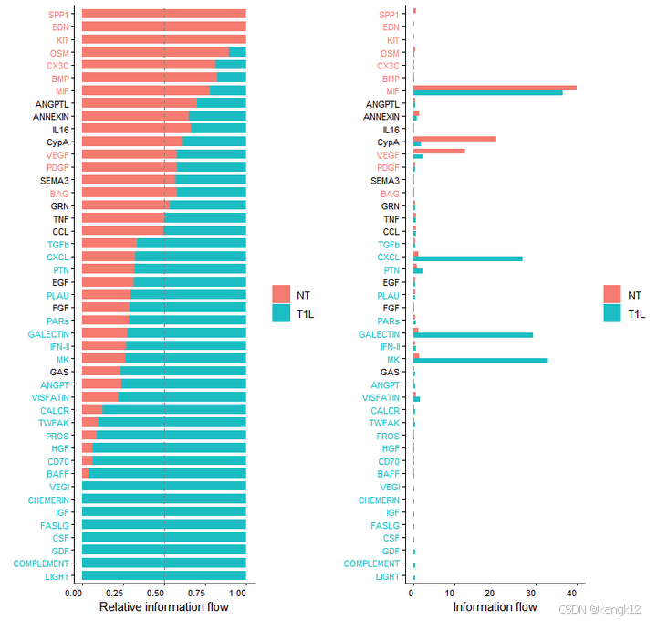

比较与每个细胞群体相关的传出和传入信号模式

R 复制代码

library(ComplexHeatmap)
i = 1
# combining all the identified signaling pathways from different datasets 
pathway.union <- union(object.list[[i]]@netP$pathways, object.list[[i+1]]@netP$pathways)
ht1 = netAnalysis_signalingRole_heatmap(object.list[[i]], pattern = "outgoing", signaling = pathway.union, title = names(object.list)[i], width = 5, height = 6)
ht2 = netAnalysis_signalingRole_heatmap(object.list[[i+1]], pattern = "outgoing", signaling = pathway.union, title = names(object.list)[i+1], width = 5, height = 6)
draw(ht1 + ht2, ht_gap = unit(0.5, "cm"))

7.识别上调和下调的信号配体-受体对

通过比较通信概率来识别功能障碍的信号

R 复制代码

netVisual_bubble(cellchat, sources.use = 4, targets.use = c(5:7),  comparison = c(1, 2), angle.x = 45)

gg1 <- netVisual_bubble(cellchat, sources.use = 4, targets.use = c(5:7),  comparison = c(1, 2), max.dataset = 2, title.name = "Increased signaling in Left", angle.x = 45, remove.isolate = T)
#> Comparing communications on a merged object
gg2 <- netVisual_bubble(cellchat, sources.use = 4, targets.use = c(5:7),  comparison = c(1, 2), max.dataset = 1, title.name = "Decreased signaling in right", angle.x = 45, remove.isolate = T)
#> Comparing communications on a merged object
gg1 + gg2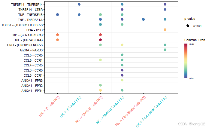

通过差异表达分析识别功能障碍性信号

对每个细胞群体在两种生物条件之间进行差异表达分析，然后根据sender细胞中配体的倍数变化和接收细胞中受体的倍数变化来获得上调和下调的信号。

R 复制代码

# 设定"实验组"
pos.dataset = "T1L"
features.name = paste0(pos.dataset, ".merged")
cellchat <- identifyOverExpressedGenes(cellchat, group.dataset = "datasets", pos.dataset = pos.dataset,
                                       features.name = features.name, only.pos = FALSE, thresh.pc = 0.1, 
                                       thresh.fc = 0.05,thresh.p = 0.05, group.DE.combined = FALSE) 

net <- netMappingDEG(cellchat, features.name = features.name, variable.all = TRUE)
net.up <- subsetCommunication(cellchat, net = net, datasets = "NT",ligand.logFC = 0.05, receptor.logFC = NULL)
net.down <- subsetCommunication(cellchat, net = net, datasets = "T1L",ligand.logFC = -0.05, receptor.logFC = NULL)

gene.up <- extractGeneSubsetFromPair(net.up, cellchat)
gene.down <- extractGeneSubsetFromPair(net.down, cellchat)

# 自定义特征和感兴趣的细胞群体找到所有显著的outgoing/incoming/both向信号
df <- findEnrichedSignaling(object.list[[2]], features = c("CCL19", "CXCL12"), idents = c("Endothelial", "CD 4"), pattern ="outgoing")

可视化

气泡图

R 复制代码

# 气泡图
pairLR.use.up = net.up[, "interaction_name", drop = F]
gg1 <- netVisual_bubble(cellchat, pairLR.use = pairLR.use.up, sources.use = 1, targets.use = c(2:9), comparison = c(1, 2),  angle.x = 90, remove.isolate = T,title.name = paste0("Up-regulated signaling in ", names(object.list)[2]))
pairLR.use.down = net.down[, "interaction_name", drop = F]
gg2 <- netVisual_bubble(cellchat, pairLR.use = pairLR.use.down, sources.use =1, targets.use = c(2:9), comparison = c(1, 2),  angle.x = 90, remove.isolate = T,title.name = paste0("Down-regulated signaling in ", names(object.list)[2]))
gg1 + gg2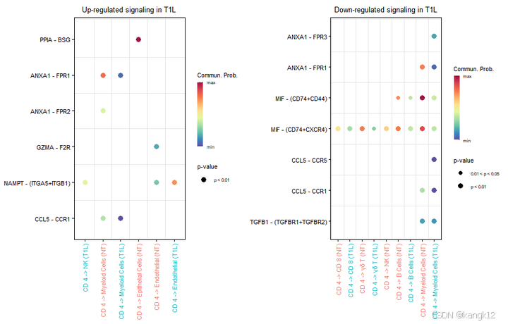

和弦图

R 复制代码

# 和弦图
# Chord diagram
par(mfrow = c(1,2), xpd=TRUE)
netVisual_chord_gene(object.list[[2]], sources.use = 1, targets.use = c(2:9), slot.name = 'net', net = net.up, lab.cex = 0.8, small.gap = 3.5, title.name = paste0("Up-regulated signaling in ", names(object.list)[2]))
netVisual_chord_gene(object.list[[1]], sources.use = 1, targets.use = c(2:9), slot.name = 'net', net = net.down, lab.cex = 0.8, small.gap = 3.5, title.name = paste0("Down-regulated signaling in ", names(object.list)[2]))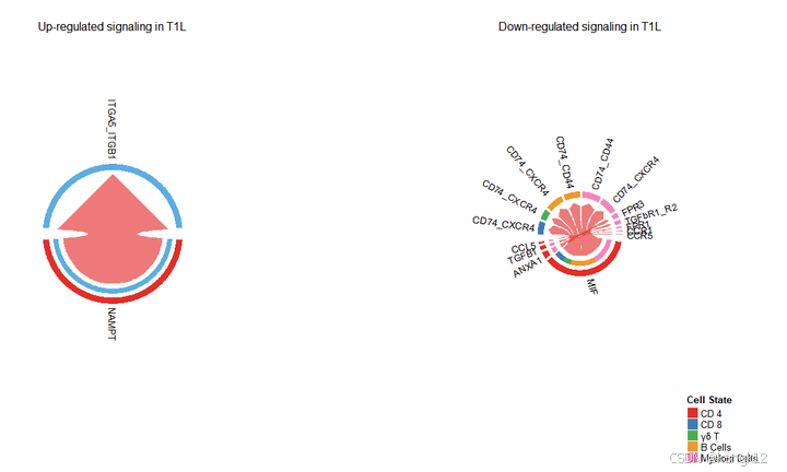

词云图

R 复制代码

# 词云图
library(wordcloud)
computeEnrichmentScore(net.down, species = 'human', variable.both = TRUE)
computeEnrichmentScore(net.up, species = 'human', variable.both = TRUE)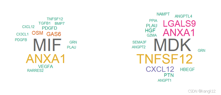

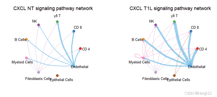
8.可视化，使用层次图、圆形图或弦图直观比较细胞间通讯

R 复制代码

pathways.show <- c("CXCL") 
weight.max <- getMaxWeight(object.list, slot.name = c("netP"), attribute = pathways.show) # control the edge weights across different datasets
par(mfrow = c(1,2), xpd=TRUE)
for (i in 1:length(object.list)) {
  netVisual_aggregate(object.list[[i]], signaling = pathways.show, layout = "circle", edge.weight.max = weight.max[1], edge.width.max = 10, signaling.name = paste(pathways.show, names(object.list)[i]))
}

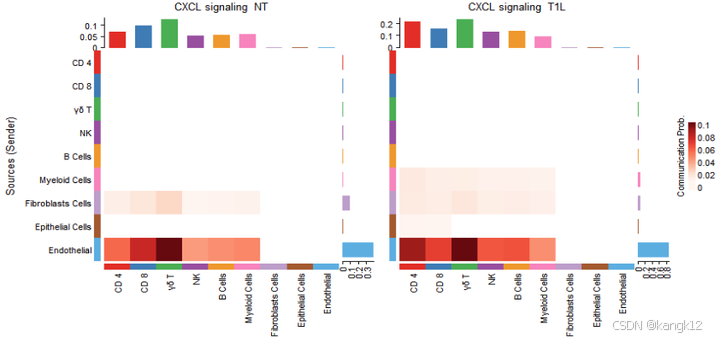
pathways.show <- c("CXCL") 
par(mfrow = c(1,2), xpd=TRUE)
ht <- list()
for (i in 1:length(object.list)) {
  ht[[i]] <- netVisual_heatmap(object.list[[i]], signaling = pathways.show, color.heatmap = "Reds",title.name = paste(pathways.show, "signaling ",names(object.list)[i]))
}
#> Do heatmap based on a single object 
#> 
#> Do heatmap based on a single object
ComplexHeatmap::draw(ht[[1]] + ht[[2]], ht_gap = unit(0.5, "cm"))

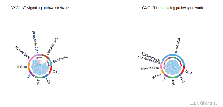
# Chord diagram
pathways.show <- c("CXCL") 
par(mfrow = c(1,2), xpd=TRUE)
for (i in 1:length(object.list)) {
  netVisual_aggregate(object.list[[i]], signaling = pathways.show, layout = "chord", signaling.name = paste(pathways.show, names(object.list)[i]))
}
# Chord diagram 的另外一种形式
# group.cellType <- c(rep("FIB", 2), rep("DC", 3), rep("TC", 4)) # grouping cell clusters into fibroblast, DC and TC cells
# names(group.cellType) <- levels(object.list[[1]]@idents)
# pathways.show <- c("CXCL") 
# par(mfrow = c(1,2), xpd=TRUE)
# for (i in 1:length(object.list)) {
#   netVisual_chord_cell(object.list[[i]], signaling = pathways.show, group = group.cellType, title.name = paste0(pathways.show, " signaling network - ", names(object.list)[i]))
# }

par(mfrow = c(1, 2), xpd=TRUE)
for (i in 1:length(object.list)) {
  netVisual_chord_gene(object.list[[i]], sources.use = 4, targets.use = c(5:6), lab.cex = 0.5, title.name = paste0("Signaling from Tm - ", names(object.list)[i]))
}

# compare all the interactions sending from fibroblast to inflamatory immune cells
# par(mfrow = c(1, 2), xpd=TRUE)
# for (i in 1:length(object.list)) {
#   netVisual_chord_gene(object.list[[i]], sources.use = c(1,2, 3, 4), targets.use = c(8,10),  title.name = paste0("Signaling received by Inflam.DC and .TC - ", names(object.list)[i]), legend.pos.x = 10)
# }

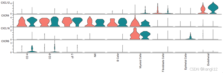
9.可视化，表达情况

R 复制代码

cellchat@meta$datasets = factor(cellchat@meta$datasets, levels = c("NT", "T1L")) # set factor level
plotGeneExpression(cellchat, signaling = "CXCL", split.by = "datasets", colors.ggplot = T, type = "violin")

参考

单细胞实战之cellchat------入门到进阶(高级篇1）-腾讯云开发者社区-腾讯云

https://htmlpreview.github.io/?https://github.com/jinworks/CellChat/blob/master/tutorial/Comparison_analysis_of_multiple_datasets.html