数据处理：下采样与SMOTE过采样

文章目录

• • 一、数据准备与标准化
  • [1. 下采样技术](#1. 下采样技术)
  • [2. SMOTE过采样技术](#2. SMOTE过采样技术)
  • [3. 模型训练与评估](#3. 模型训练与评估)
  • • 超参数调优
    • 混淆矩阵可视化函数
    • 最终模型训练与评估
  • 二、技术对比与选择建议

---

一、数据准备与标准化

• 首先，我们需要加载并预处理数据。以下是完整的数据准备代码：

import numpy as np
from numpy.ma import negative
from sklearn.model_selection import train_test_split, cross_val_score
from sklearn.preprocessing import StandardScaler
import pandas as pd
import matplotlib.pyplot as plt
from pylab import mpl
from sklearn.linear_model import LogisticRegression
from sklearn import metrics
from imblearn.over_sampling import SMOTE
import time

# 读取数据并标准化
data = pd.read_csv(r"creditcard.csv")
scaler = StandardScaler()
data["Amount"] = scaler.fit_transform(data[["Amount"]])
data = data.drop(["Time"], axis=1)

# 设置中文字体
mpl.rcParams["font.sans-serif"] = ["Microsoft YaHei"]
mpl.rcParams["axes.unicode_minus"] = False

# 可视化正负样本分布
labels_count = pd.value_counts(data["Class"])
print(labels_count)
plt.title("正负例样本数")
plt.xlabel("类别")
plt.ylabel("频数")
labels_count.plot(kind='bar')
plt.show()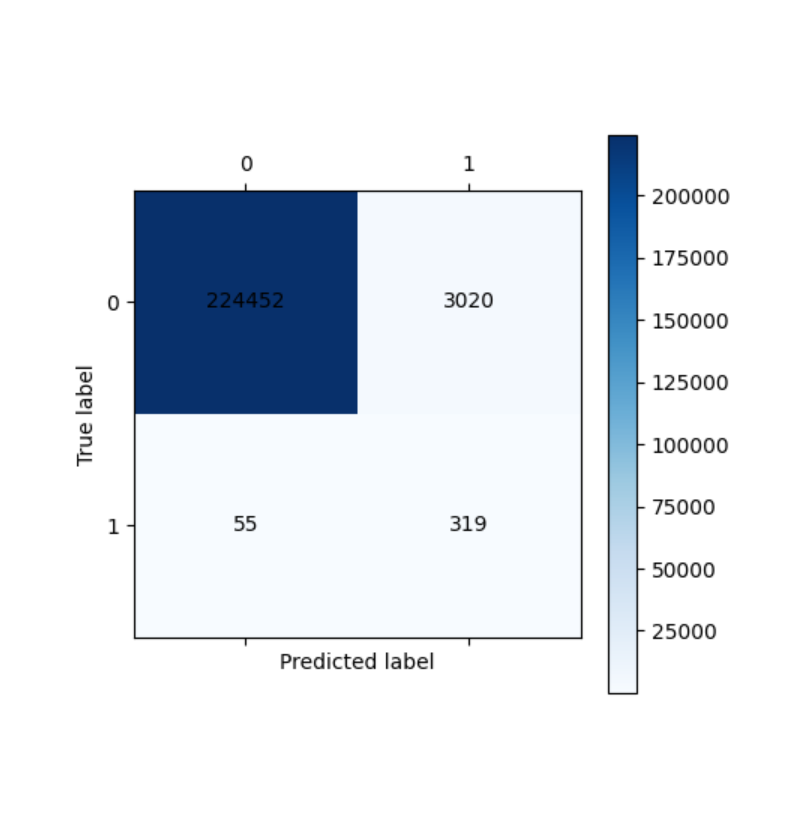

• 这段代码首先加载信用卡交易数据，对交易金额进行标准化处理，并移除时间列。通过可视化，我们可以清楚地看到正负样本（正常交易与欺诈交易）的情况。

1. 下采样技术

• 下采样是通过减少多数类样本来平衡数据集的方法。在信用卡欺诈检测中，正常交易样本（多数类）远多于欺诈交易样本（少数类）。下采样随机选择与少数类数量相同的多数类样本，从而创建平衡的训练集。

# 创建训练数据副本
data_train = data.copy()

# 分离正负样本
positive_eg = data_train[data_train["Class"] == 0]
negative_eg = data_train[data_train["Class"] == 1]

# 下采样：从多数类中随机抽取与少数类相同数量的样本
positive_eg = positive_eg.sample(len(negative_eg))

# 合并平衡后的数据集
data_c = pd.concat([positive_eg, negative_eg])

# 准备特征和标签
column_names = ['V1', 'V2', 'V3', 'V4', 'V5', 'V6', 'V7', 'V8', 'V9', 'V10',
                'V11', 'V12', 'V13', 'V14', 'V15', 'V16', 'V17', 'V18', 'V19',
                'V20', 'V21', 'V22', 'V23', 'V24', 'V25', 'V26', 'V27', 'V28', 'Amount']

x_whole = data_c[column_names]
y_whole = data_c[["Class"]]

# 划分训练集和测试集
x_train_w, x_test_w, y_train_w, y_test_w = train_test_split(x_whole, y_whole, train_size=0.3, random_state=1000)

# 使用逻辑回归模型
lr = LogisticRegression(C=0.01)
lr.fit(x_train_w, y_train_w)

# 预测和评估
test_predicted = lr.predict(x_test_w)
result = lr.score(x_test_w, y_test_w)

print(metrics.classification_report(y_test_w, test_predicted))

• 下采样的优点是简单易实现，计算效率高，但缺点是会丢失大量多数类样本的信息，可能降低模型性能。

2. SMOTE过采样技术

• SMOTE（Synthetic Minority Over-sampling Technique）是一种更先进的过采样技术，它通过生成合成样本来增加少数类样本数量，而不是简单复制现有样本。

# 使用完整不平衡数据集
x_whole = data[column_names]
y_whole = data[["Class"]]

# 划分训练集和测试集
x_train, x_test, y_train, y_test = train_test_split(x_whole, y_whole, train_size=0.2, random_state=1000)

# 应用SMOTE过采样
oversampler = SMOTE(random_state=0)
os_x_train, os_y_train = oversampler.fit_resample(x_train, y_train)

• SMOTE的工作原理是在少数类样本之间进行插值，生成新的合成样本。具体来说，对于每个少数类样本，SMOTE会：

1. 找到该样本的k个最近邻少数类样本
2. 随机选择其中一个邻居
3. 在原始样本和邻居之间的连线上随机选择一个点作为新样本

3. 模型训练与评估

超参数调优

• 使用交叉验证来寻找最优的正则化参数C：

scores = []
c_param_range = [0.01, 0.1, 1, 10, 100]
z = 1

for i in c_param_range:
    start_time = time.time()
    lr = LogisticRegression(C=i, penalty="l2", solver="lbfgs", max_iter=1000)
    score = cross_val_score(lr, os_x_train, os_y_train, cv=8, scoring="recall")
    score_mean = sum(score) / len(score)
    scores.append(score_mean)
    end_time = time.time()
    
    print("第{}次...".format(z))
    print("time spend:{:.2f}".format(end_time - start_time))
    print("recall:{}".format(score_mean))
    z += 1

best_c = c_param_range[np.argmax(scores)]
print(f"........最优惩罚因子为:{best_c}........")

混淆矩阵可视化函数

def cm_plot(y, yp):
    from sklearn.metrics import confusion_matrix
    import matplotlib.pyplot as plt

    cm = confusion_matrix(y, yp)
    plt.matshow(cm, cmap=plt.cm.Blues)
    plt.colorbar()

    for x in range(len(cm)):
        for y in range(len(cm)):
            plt.annotate(cm[x, y], xy=(y, x), horizontalalignment='center',
                         verticalalignment='center')
            plt.ylabel('True label')
            plt.xlabel('Predicted label')

    return plt

最终模型训练与评估

# 使用最优参数训练模型
lr = LogisticRegression(C=best_c, penalty="l2", max_iter=1000)
lr.fit(os_x_train, os_y_train)

# 训练集预测和评估
train_predicted = lr.predict(os_x_train)
print(metrics.classification_report(os_y_train, train_predicted, digits=6))
cm_plot(os_y_train, train_predicted).show()

# 测试集预测和评估
test_predicted = lr.predict(x_test)
print(metrics.classification_report(y_test, test_predicted, digits=6))
cm_plot(y_test, test_predicted).show()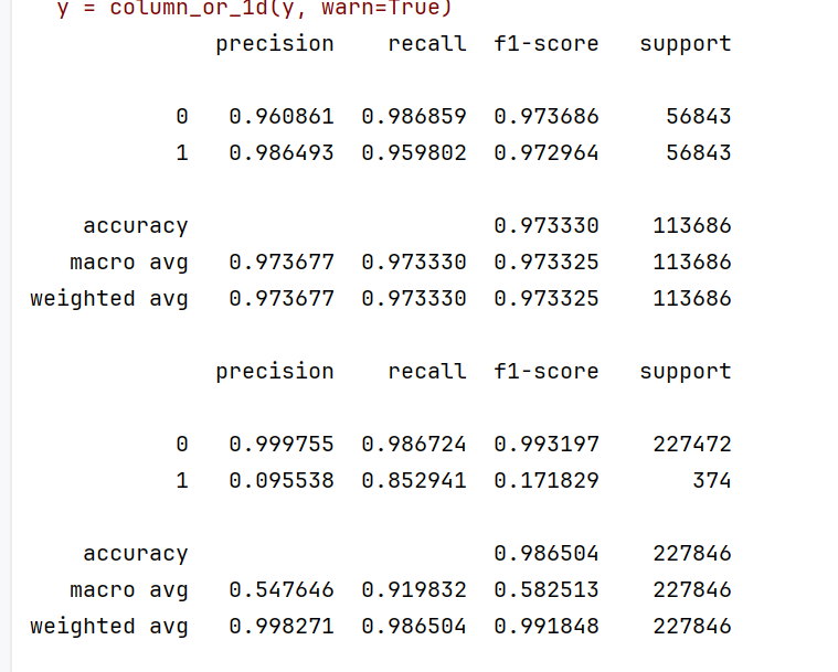

二、技术对比与选择建议

1. 下采样

   • 优点：计算效率高，适用于大规模数据集
   • 缺点：丢失大量多数类信息，可能降低模型泛化能力
   • 适用场景：计算资源有限，多数类样本冗余度高

2. SMOTE过采样

   • 优点：保留所有样本信息，生成多样化的合成样本
   • 缺点：可能生成不现实的样本，计算成本较高
   • 适用场景：少数类样本非常稀少，需要保留所有原始信息

在实际应用中，建议根据具体问题和数据特性选择合适的采样技术。同时，通过合理的数据预处理和采样技术，我们可以显著提高模型在不平衡数据集上的性能，特别是在召回率这一关键指标上。