3000个样本的时候,训练得到的结果:
import torch
import torch.nn as nn
import torch.nn.functional as F
import torch.optim as optim
from torch.utils.data import DataLoader, TensorDataset
import pandas as pd
import numpy as np
from sklearn.model_selection import train_test_split
import os
import gc

# ----------------------------
# 1. 参数配置
# ----------------------------
DEVICE = torch.device('cuda' if torch.cuda.is_available() else 'cpu')
print(f"Using device: {DEVICE}")

INPUT_LENGTH = 3000  # 每个样本长度
NUM_SAMPLES = 3000  # 总样本数
BATCH_SIZE = 16  # 减小批处理大小
GRAD_ACCUM_STEPS = 2  # 梯度累积步数
EPOCHS = 50  # 训练次数
LEARNING_RATE = 1e-3

# ----------------------------
# 2. 读取 Excel 数据
# ----------------------------
print("Loading data from Excel...")
train_df = pd.read_excel('train_data.xlsx', header=None)  # (3000, 3000)
label_df = pd.read_excel('label_data.xlsx', header=None)  # (3000, 2)

# 转为 numpy
X = train_df.values.astype(np.float32)  # shape: (3000, 3000)
y = label_df.values.astype(np.float32)  # shape: (3000, 2)

assert X.shape == (NUM_SAMPLES, INPUT_LENGTH), f"Expected ({NUM_SAMPLES}, {INPUT_LENGTH}), got {X.shape}"
assert y.shape[1] == 2, "Label should have 2 columns: [slice_width, sampling_interval]"

# ----------------------------
# 3. 划分训练/验证集 (80% / 20%)
# ----------------------------
X_train, X_val, y_train, y_val = train_test_split(
    X, y, test_size=0.2, random_state=42
)

# 转为 PyTorch 张量
X_train = torch.from_numpy(X_train)
y_train = torch.from_numpy(y_train)
X_val = torch.from_numpy(X_val)
y_val = torch.from_numpy(y_val)

# 创建 Dataset 和 DataLoader
train_dataset = TensorDataset(X_train, y_train)
val_dataset = TensorDataset(X_val, y_val)

train_loader = DataLoader(train_dataset, batch_size=BATCH_SIZE, shuffle=True)
val_loader = DataLoader(val_dataset, batch_size=BATCH_SIZE, shuffle=False)


# ----------------------------
# 4. 定义改进的参数回归网络
# ----------------------------
class ParamRegressionModule(nn.Module):
    def __init__(self, input_length=3000):
        super().__init__()

        # 第一层卷积:1 → 64通道
        self.conv1 = nn.Conv1d(1, 64, kernel_size=16, padding=8)  # padding='same'
        self.bn1 = nn.BatchNorm1d(64)

        # 第二层卷积:64 → 128通道
        self.conv2 = nn.Conv1d(64, 128, kernel_size=16, padding=8)
        self.bn2 = nn.BatchNorm1d(128)

        # 第三层卷积:128 → 64通道
        self.conv3 = nn.Conv1d(128, 64, kernel_size=16, padding=8)
        self.bn3 = nn.BatchNorm1d(64)

        # 池化层
        self.pool1 = nn.MaxPool1d(2)
        self.pool2 = nn.MaxPool1d(2)
        self.pool3 = nn.MaxPool1d(2)

        # 全局池化
        self.global_pool = nn.AdaptiveAvgPool1d(50)  # 将长度池化到固定值50

        # Dropout
        self.dropout = nn.Dropout(0.3)

        # 计算全连接层输入维度
        self.fc_input_dim = 64 * 50  # 64通道 * 50长度

        # 全连接层
        self.fc = nn.Sequential(
            nn.Linear(self.fc_input_dim, 128),
            nn.ReLU(),
            nn.Dropout(0.3),
            nn.Linear(128, 64),
            nn.ReLU(),
            nn.Dropout(0.2),
            nn.Linear(64, 2)
        )

        # 初始化权重
        self._initialize_weights()

    def _initialize_weights(self):
        for m in self.modules():
            if isinstance(m, nn.Conv1d):
                nn.init.kaiming_normal_(m.weight, mode='fan_out', nonlinearity='relu')
                if m.bias is not None:
                    nn.init.constant_(m.bias, 0)
            elif isinstance(m, nn.BatchNorm1d):
                nn.init.constant_(m.weight, 1)
                nn.init.constant_(m.bias, 0)
            elif isinstance(m, nn.Linear):
                nn.init.normal_(m.weight, 0, 0.01)
                nn.init.constant_(m.bias, 0)

    def forward(self, x):
        # 输入形状: (batch_size, input_length)
        x = x.unsqueeze(1)  # (B, 1, L)

        # 第一层
        x = F.relu(self.bn1(self.conv1(x)))
        x = self.pool1(x)
        x = self.dropout(x)  # (B, 64, L/2)

        # 第二层
        x = F.relu(self.bn2(self.conv2(x)))
        x = self.pool2(x)
        x = self.dropout(x)  # (B, 128, L/4)

        # 第三层
        x = F.relu(self.bn3(self.conv3(x)))
        x = self.pool3(x)  # (B, 64, L/8)

        # 全局池化到固定长度
        x = self.global_pool(x)  # (B, 64, 50)

        # 展平
        x = x.view(x.size(0), -1)  # (B, 64*50)

        # 全连接层
        x = self.fc(x)

        return x


# ----------------------------
# 5. 初始化模型、损失函数、优化器
# ----------------------------
model = ParamRegressionModule(input_length=INPUT_LENGTH).to(DEVICE)
criterion = nn.MSELoss()
optimizer = optim.Adam(model.parameters(), lr=LEARNING_RATE)

# 学习率调度器(移除了verbose参数)
scheduler = optim.lr_scheduler.ReduceLROnPlateau(
    optimizer, mode='min', factor=0.5, patience=5
)

# 打印模型信息
print("Model architecture:")
print(model)
print(f"Total parameters: {sum(p.numel() for p in model.parameters())}")
print(f"Trainable parameters: {sum(p.numel() for p in model.parameters() if p.requires_grad)}")

# ----------------------------
# 6. 训练循环(使用梯度累积)
# ----------------------------
print(f"\nStart training with batch size {BATCH_SIZE} and grad accumulation {GRAD_ACCUM_STEPS}...")
print(f"Effective batch size: {BATCH_SIZE * GRAD_ACCUM_STEPS}")

# 用于记录训练历史
train_history = []
val_history = []
best_val_loss = float('inf')
best_epoch = 0

for epoch in range(EPOCHS):
    # 训练阶段
    model.train()
    train_loss = 0.0
    optimizer.zero_grad()  # 在epoch开始时清零梯度

    for batch_idx, (batch_x, batch_y) in enumerate(train_loader):
        batch_x = batch_x.to(DEVICE)
        batch_y = batch_y.to(DEVICE)

        # 前向传播
        outputs = model(batch_x)
        loss = criterion(outputs, batch_y)

        # 梯度累积:标准化损失
        loss = loss / GRAD_ACCUM_STEPS
        loss.backward()

        train_loss += loss.item() * batch_x.size(0) * GRAD_ACCUM_STEPS

        # 每 GRAD_ACCUM_STEPS 步更新一次参数
        if (batch_idx + 1) % GRAD_ACCUM_STEPS == 0:
            optimizer.step()
            optimizer.zero_grad()

            # 清理GPU缓存
            if torch.cuda.is_available():
                torch.cuda.empty_cache()

    # 如果还有未更新的梯度,再更新一次
    if len(train_loader) % GRAD_ACCUM_STEPS != 0:
        optimizer.step()
        optimizer.zero_grad()

    # 计算平均训练损失
    train_loss /= len(train_loader.dataset)
    train_history.append(train_loss)

    # 验证阶段
    model.eval()
    val_loss = 0.0
    with torch.no_grad():
        for batch_x, batch_y in val_loader:
            batch_x = batch_x.to(DEVICE)
            batch_y = batch_y.to(DEVICE)
            outputs = model(batch_x)
            loss = criterion(outputs, batch_y)
            val_loss += loss.item() * batch_x.size(0)

            # 清理GPU缓存
            if torch.cuda.is_available():
                torch.cuda.empty_cache()

    # 计算平均验证损失
    val_loss /= len(val_loader.dataset)
    val_history.append(val_loss)

    # 更新学习率
    scheduler.step(val_loss)

    # 打印进度
    current_lr = optimizer.param_groups[0]['lr']
    print(f"Epoch [{epoch + 1:03d}/{EPOCHS}] | "
          f"Train Loss: {train_loss:.6f} | "
          f"Val Loss: {val_loss:.6f} | "
          f"LR: {current_lr:.2e}")

    # 保存最佳模型
    if val_loss < best_val_loss:
        best_val_loss = val_loss
        best_epoch = epoch + 1
        torch.save({
            'epoch': epoch,
            'model_state_dict': model.state_dict(),
            'optimizer_state_dict': optimizer.state_dict(),
            'train_loss': train_loss,
            'val_loss': val_loss,
            'train_history': train_history,
            'val_history': val_history
        }, 'best_model.pth')
        print(f"  -> New best model saved at epoch {best_epoch} with val loss: {val_loss:.6f}")

    # 强制垃圾回收
    gc.collect()
    if torch.cuda.is_available():
        torch.cuda.empty_cache()

# ----------------------------
# 7. 保存最终模型
# ----------------------------
torch.save({
    'epoch': EPOCHS,
    'model_state_dict': model.state_dict(),
    'optimizer_state_dict': optimizer.state_dict(),
    'train_history': train_history,
    'val_history': val_history
}, 'final_model.pth')
print(f"\nFinal model saved as 'final_model.pth'")
print(f"Best model at epoch {best_epoch} with val loss: {best_val_loss:.6f}")

# 绘制训练曲线(可选)
try:
    import matplotlib.pyplot as plt

    plt.figure(figsize=(12, 8))

    # 绘制损失曲线
    plt.subplot(2, 1, 1)
    plt.plot(train_history, label='Train Loss', linewidth=2)
    plt.plot(val_history, label='Val Loss', linewidth=2)
    plt.xlabel('Epoch')
    plt.ylabel('Loss')
    plt.title('Training History')
    plt.legend()
    plt.grid(True)

    # 标记最佳epoch
    plt.axvline(x=best_epoch - 1, color='r', linestyle='--', alpha=0.5, label=f'Best Epoch: {best_epoch}')
    plt.legend()

    # 绘制损失对数值
    plt.subplot(2, 1, 2)
    plt.semilogy(train_history, label='Train Loss', linewidth=2)
    plt.semilogy(val_history, label='Val Loss', linewidth=2)
    plt.xlabel('Epoch')
    plt.ylabel('Loss (log scale)')
    plt.title('Training History (Log Scale)')
    plt.legend()
    plt.grid(True)

    plt.tight_layout()
    plt.savefig('training_history.png', dpi=300, bbox_inches='tight')
    plt.show()
    print("Training history plot saved as 'training_history.png'")

except ImportError:
    print("Matplotlib not installed. Skipping plot.")

print("\nTraining completed!")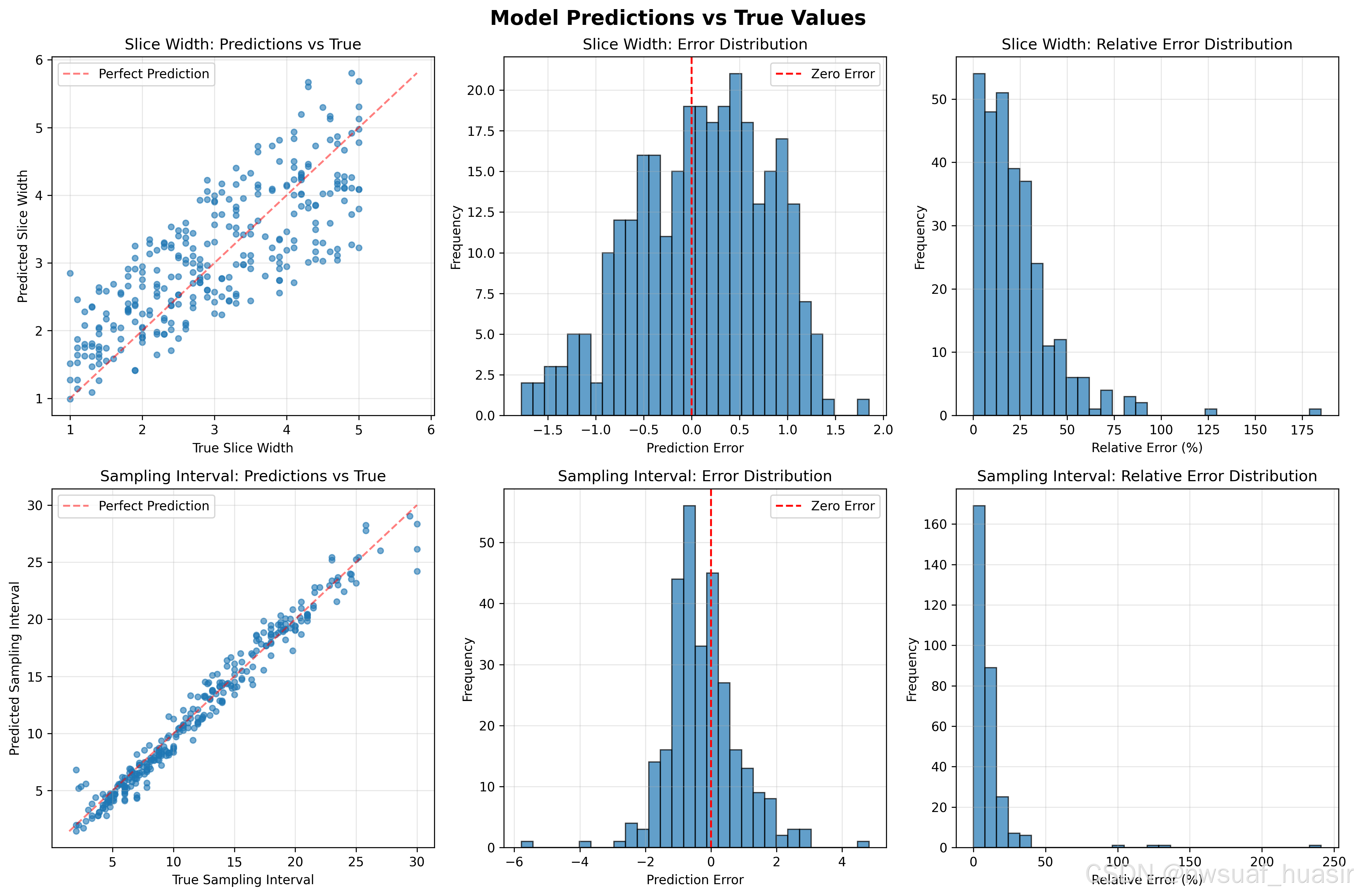
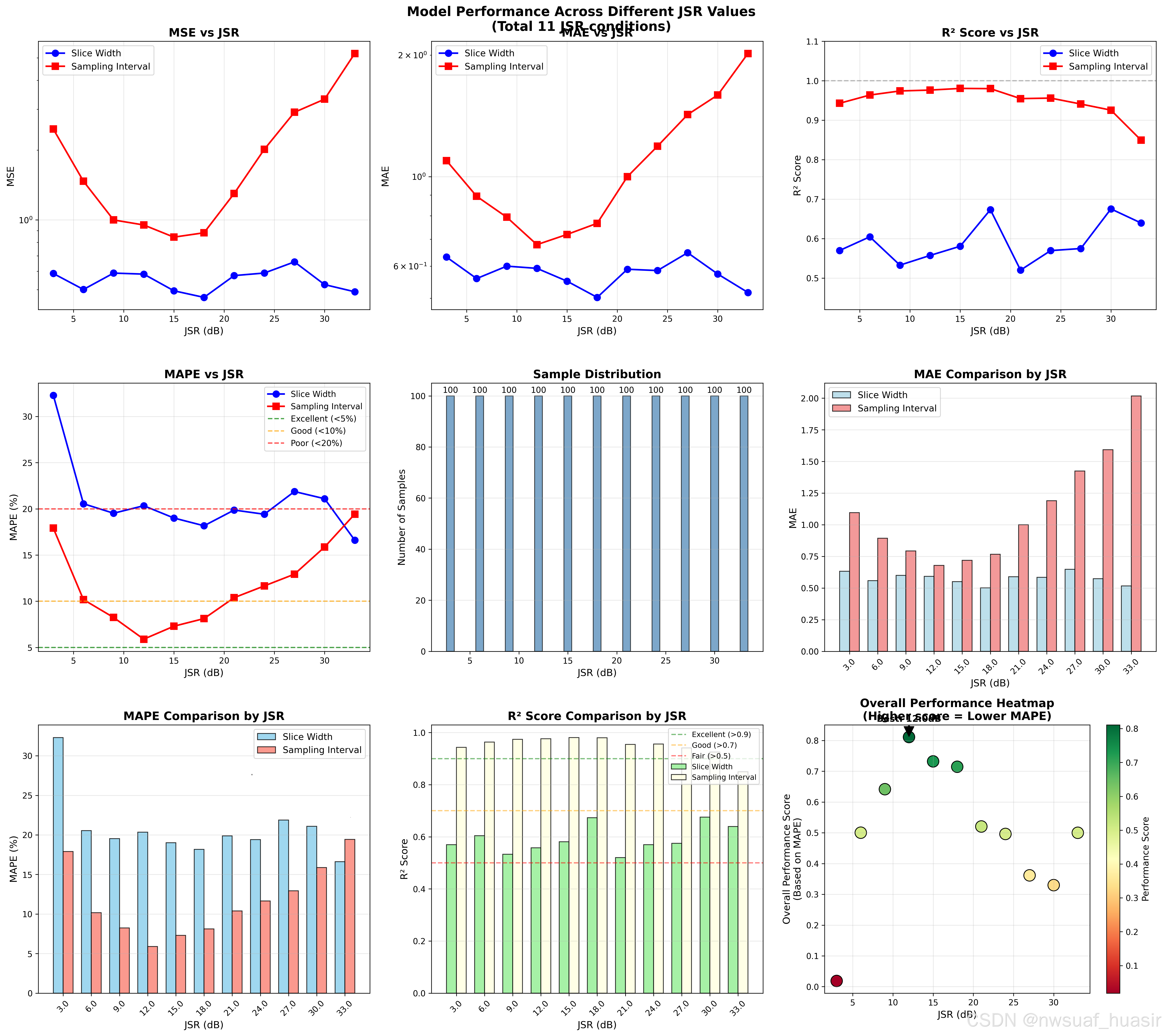
每种JSR有100个样本进行预测,得到的结果:
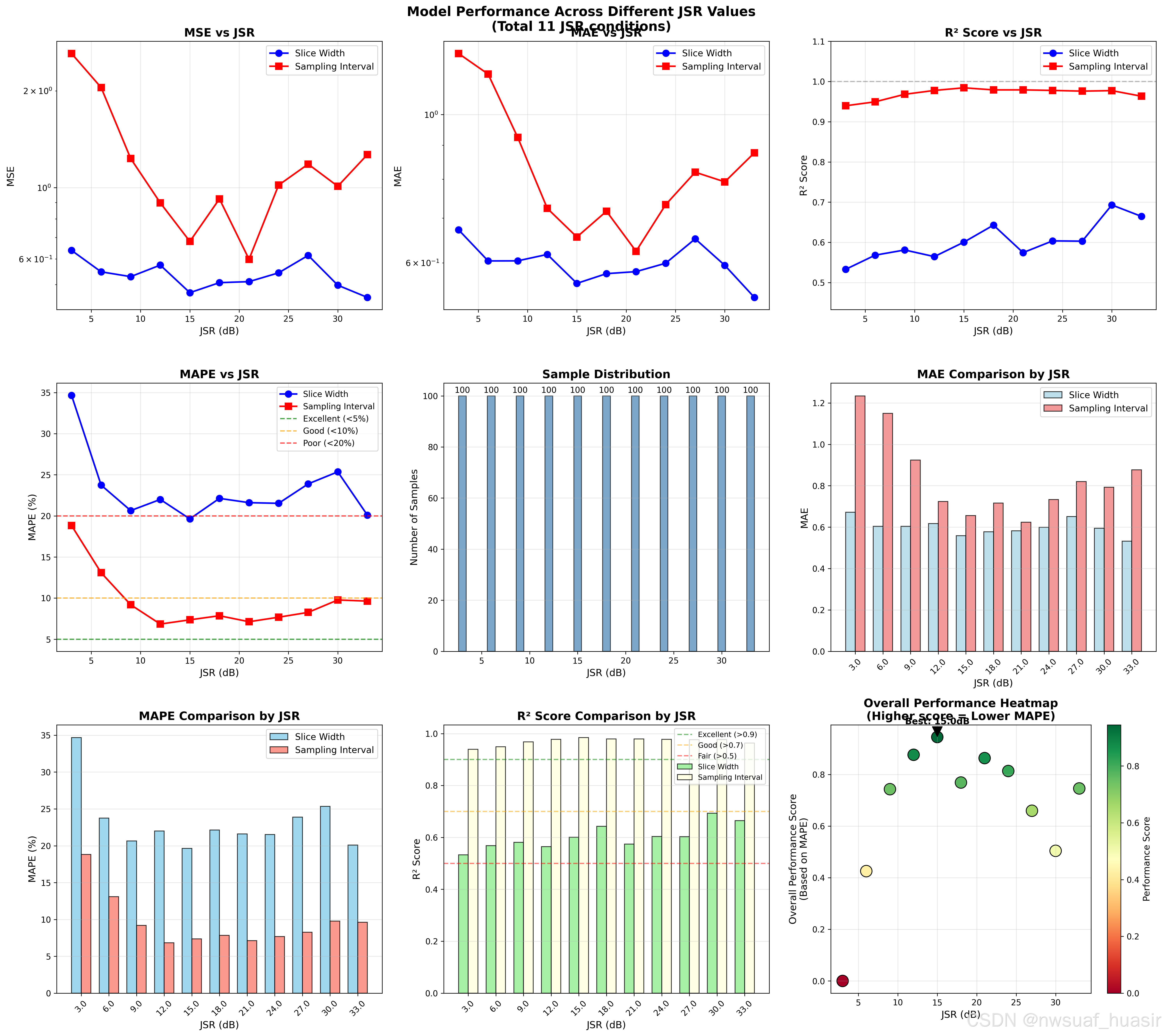
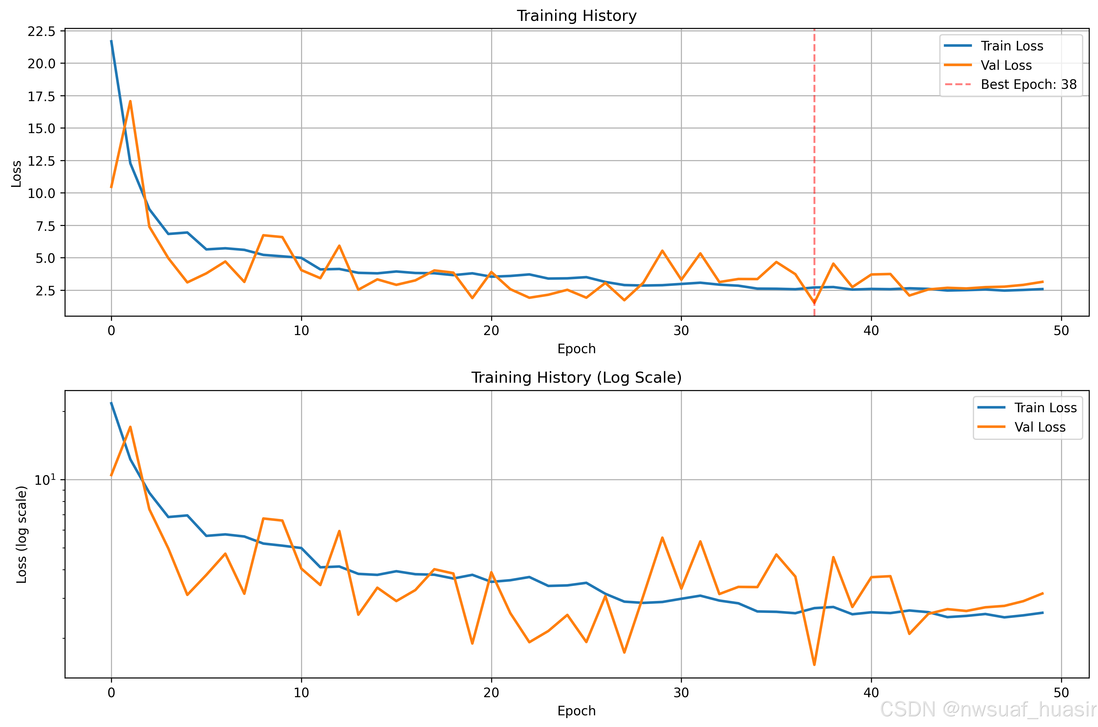
将样本增加至5500,得到的训练过程的曲线如下所示:
最终的结果: