【OpenCV】Python图像处理之仿射变换

仿射变换（Affine Transformation）是一种保持图像平行性 和共线性 的几何变换，核心是通过线性变换（缩放、旋转、剪切）与平移变换的组合，改变图像的位置、姿态和尺寸，但不改变图形的平行关系（如平行线变换后仍平行）。OpenCV 中通过 cv2.warpAffine() 函数实现仿射变换，需先构造仿射变换矩阵，广泛用于图像校正、姿态调整、视角变换等场景。

一、核心原理

1. 仿射变换的数学表达

对于图像中任意像素点 (x, y)，仿射变换后映射到新坐标 (x', y')，其数学公式为：

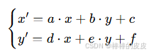
用矩阵形式表示为：

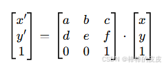
其中：

• 2×3 矩阵 [[a,b,c],[d,e,f]] 为仿射变换矩阵 （OpenCV 中需用 numpy.ndarray 表示， dtype 为 np.float32）；
• 前 2×2 子矩阵 [[a,b],[d,e]] 负责线性变换（缩放、旋转、剪切）；
• 最后一列 [c,f] 负责平移变换（x 方向平移 c，y 方向平移 f）。

2. 仿射变换的三大基础操作

仿射变换可分解为三种基础变换的组合，也可直接通过这三种变换构造矩阵：

基础变换	作用	变换矩阵特点
平移（Translation）	图像沿 x/y 轴移动	前 2×2 为单位矩阵 [[1,0],[0,1]]，平移量 [c,f]
旋转（Rotation）	图像绕原点 / 特定点旋转	前 2×2 为旋转矩阵 [[cosθ, -sinθ],[sinθ, cosθ]]，可结合平移实现绕任意点旋转
缩放（Scaling）	图像沿 x/y 轴缩放	前 2×2 为对角矩阵 [[sx,0],[0,sy]]（sx/sy 为宽 / 高缩放比例）

3. 仿射变换矩阵的构造方式

OpenCV 提供两种核心构造方法，无需手动计算矩阵：

1. 通过三点映射构造 ：已知原图中 3 个非共线点及其变换后的对应点，用 cv2.getAffineTransform(src_pts, dst_pts) 自动计算变换矩阵（最常用）；
2. 手动构造：直接根据平移、旋转、缩放的数学公式创建 2×3 矩阵（适合简单变换）。

二、核心函数详解

1. cv2.getAffineTransform()：通过三点映射生成变换矩阵

函数原型

cv2.getAffineTransform(src_pts, dst_pts)

参数说明

参数	含义	要求
src_pts	原图中 3 个非共线点的坐标	格式为 np.float32([[x1,y1], [x2,y2], [x3,y3]])
dst_pts	变换后对应 3 个点的坐标	格式与 src_pts 一致，数量必须为 3

返回值

2×3 仿射变换矩阵（np.float32 类型）。

2. cv2.warpAffine()：应用仿射变换

函数原型

cv2.warpAffine(src, M, dsize, dst=None, flags=None, borderMode=None, borderValue=None)

参数说明

参数	含义	注意事项
src	输入图像	单通道 / 多通道均可（灰度图 / 彩色图）
M	仿射变换矩阵	必须是 2×3 的 np.float32 矩阵
dsize	输出图像尺寸	格式为 (width, height)（与 OpenCV 图像 shape 相反）
flags	插值算法（可选）	默认 cv2.INTER_LINEAR，缩小用 INTER_AREA，高质量放大用 INTER_CUBIC
borderMode	边界填充模式（可选）	默认 cv2.BORDER_CONSTANT（常数填充），也可设为 BORDER_REPLICATE（复制边界）
borderValue	边界填充值（可选）	仅 borderMode=BORDER_CONSTANT 有效，默认黑色（0），彩色图用 (b,g,r) 格式

返回值

变换后的输出图像（numpy.ndarray 类型）。

三、完整实现代码（多种场景）

1. 基础场景：通过三点映射实现任意仿射变换

已知原图 3 个点和目标点，自动计算矩阵实现变换（如校正倾斜图像）：

import cv2
import numpy as np
import matplotlib.pyplot as plt

# 1. 读取图像
img = cv2.imread("lena.jpg")
if img is None:
    print("无法读取图像，请检查路径！")
    exit()
h, w = img.shape[:2]
img_rgb = cv2.cvtColor(img, cv2.COLOR_BGR2RGB)  # 转为RGB用于matplotlib显示

# 2. 定义原图3个点和变换后对应3个点（非共线）
# 原图中选择3个特征点（如左上角、右上角、左下角）
src_pts = np.float32([[50, 50], [200, 50], [50, 200]])
# 变换后目标点（示例：向右倾斜、向下平移）
dst_pts = np.float32([[50, 50], [250, 80], [30, 220]])

# 3. 计算仿射变换矩阵
M = cv2.getAffineTransform(src_pts, dst_pts)

# 4. 应用仿射变换（输出尺寸与原图一致）
img_affine = cv2.warpAffine(img, M, (w, h), flags=cv2.INTER_LINEAR, borderValue=(255,255,255))
img_affine_rgb = cv2.cvtColor(img_affine, cv2.COLOR_BGR2RGB)

# 5. 绘制特征点（可视化对应关系）
for (x, y) in src_pts.astype(int):
    cv2.circle(img_rgb, (x, y), 5, (255, 0, 0), -1)  # 原图点：蓝色
for (x, y) in dst_pts.astype(int):
    cv2.circle(img_affine_rgb, (x, y), 5, (0, 255, 0), -1)  # 目标点：绿色

# 6. 显示结果
plt.figure(figsize=(12, 6))
plt.subplot(1, 2, 1)
plt.imshow(img_rgb)
plt.title("Original Image (Blue Points)")
plt.axis("off")
plt.subplot(1, 2, 2)
plt.imshow(img_affine_rgb)
plt.title("Affine Transformation (Green Points)")
plt.axis("off")
plt.tight_layout()
plt.show()

2. 常用场景：手动构造矩阵实现平移、旋转、缩放

（1）平移变换（沿 x 轴右移 100 像素，y 轴下移 50 像素）

import cv2
import numpy as np
import matplotlib.pyplot as plt

img = cv2.imread("lena.jpg")
h, w = img.shape[:2]
img_rgb = cv2.cvtColor(img, cv2.COLOR_BGR2RGB)

# 构造平移矩阵：[[1,0,c],[0,1,f]]，c=x平移量，f=y平移量
tx, ty = 100, 50  # x右移100，y下移50
M_translate = np.float32([[1, 0, tx], [0, 1, ty]])

# 应用变换（输出尺寸可适当放大，避免图像被截断）
img_translate = cv2.warpAffine(img, M_translate, (w + tx, h + ty), borderValue=(255,255,255))
img_translate_rgb = cv2.cvtColor(img_translate, cv2.COLOR_BGR2RGB)

# 显示
plt.figure(figsize=(12, 6))
plt.subplot(1, 2, 1)
plt.imshow(img_rgb)
plt.title(f"Original ({h}×{w})")
plt.axis("off")
plt.subplot(1, 2, 2)
plt.imshow(img_translate_rgb)
plt.title(f"Translated (x+100, y+50) ({img_translate.shape[0]}×{img_translate.shape[1]})")
plt.axis("off")
plt.show()

2）旋转变换（绕图像中心旋转 45°，缩放比例 0.8）

旋转矩阵需结合平移（先将旋转中心移至原点，旋转后再移回原位置），公式如下：

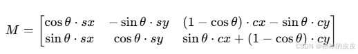
其中：θ 为旋转角度（弧度），sx/sy 为缩放比例，(cx, cy) 为旋转中心。

import cv2
import numpy as np
import matplotlib.pyplot as plt

img = cv2.imread("lena.jpg")
h, w = img.shape[:2]
img_rgb = cv2.cvtColor(img, cv2.COLOR_BGR2RGB)

# 旋转参数
angle = 45  # 旋转角度（度）
scale = 0.8  # 旋转时的缩放比例
cx, cy = w // 2, h // 2  # 旋转中心（图像中心）

# 计算旋转矩阵（OpenCV内置函数，无需手动计算）
M_rotate = cv2.getRotationMatrix2D((cx, cy), angle, scale)

# 应用旋转（输出尺寸可按旋转后的边界调整，避免截断）
img_rotate = cv2.warpAffine(img, M_rotate, (w, h), flags=cv2.INTER_CUBIC, borderValue=(255,255,255))
img_rotate_rgb = cv2.cvtColor(img_rotate, cv2.COLOR_BGR2RGB)

# 显示
plt.figure(figsize=(12, 6))
plt.subplot(1, 2, 1)
plt.imshow(img_rgb)
plt.title(f"Original ({h}×{w})")
plt.axis("off")
plt.subplot(1, 2, 2)
plt.imshow(img_rotate_rgb)
plt.title(f"Rotated {angle}° (scale={scale})")
plt.axis("off")
plt.show()

（3）缩放变换（宽度缩放 1.5 倍，高度缩放 0.8 倍）

import cv2
import numpy as np
import matplotlib.pyplot as plt

img = cv2.imread("lena.jpg")
h, w = img.shape[:2]
img_rgb = cv2.cvtColor(img, cv2.COLOR_BGR2RGB)

# 构造缩放矩阵：[[sx,0,0],[0,sy,0]]，sx=宽度缩放比，sy=高度缩放比
sx, sy = 1.5, 0.8
M_scale = np.float32([[sx, 0, 0], [0, sy, 0]])

# 应用缩放（输出尺寸=原图尺寸×缩放比）
new_w, new_h = int(w * sx), int(h * sy)
img_scale = cv2.warpAffine(img, M_scale, (new_w, new_h), flags=cv2.INTER_CUBIC)
img_scale_rgb = cv2.cvtColor(img_scale, cv2.COLOR_BGR2RGB)

# 显示
plt.figure(figsize=(12, 6))
plt.subplot(1, 2, 1)
plt.imshow(img_rgb)
plt.title(f"Original ({h}×{w})")
plt.axis("off")
plt.subplot(1, 2, 2)
plt.imshow(img_scale_rgb)
plt.title(f"Scaled (sx={sx}, sy={sy}) ({new_h}×{new_w})")
plt.axis("off")
plt.show()

3. 实用场景：图像校正（倾斜文档校正）

通过选择文档的四个角点（先取 3 个计算仿射矩阵），校正倾斜的文档图像：

import cv2
import numpy as np
import matplotlib.pyplot as plt

def correct_skew_image(img, src_pts, target_size):
    """
    校正倾斜图像（仿射变换）
    :param img: 输入倾斜图像
    :param src_pts: 原图中文档的3个角点（np.float32）
    :param target_size: 校正后目标尺寸 (width, height)
    :return: 校正后的图像
    """
    # 定义校正后目标点（文档的三个角点：左上角、右上角、左下角）
    dst_pts = np.float32([[0, 0], [target_size[0]-1, 0], [0, target_size[1]-1]])
    # 计算仿射矩阵
    M = cv2.getAffineTransform(src_pts, dst_pts)
    # 应用变换
    corrected_img = cv2.warpAffine(img, M, target_size, flags=cv2.INTER_CUBIC, borderValue=(255,255,255))
    return corrected_img

# 1. 读取倾斜文档图像
img_skew = cv2.imread("skew_document.jpg")
if img_skew is None:
    print("无法读取倾斜图像，请检查路径！")
    exit()
h, w = img_skew.shape[:2]
img_skew_rgb = cv2.cvtColor(img_skew, cv2.COLOR_BGR2RGB)

# 2. 手动选择原图中3个角点（可通过图像查看工具获取坐标）
src_pts = np.float32([[60, 80], [420, 70], [50, 500]])  # 示例坐标，需根据实际图像调整

# 3. 校正图像（目标尺寸：宽400，高550）
target_size = (400, 550)
img_corrected = correct_skew_image(img_skew, src_pts, target_size)
img_corrected_rgb = cv2.cvtColor(img_corrected, cv2.COLOR_BGR2RGB)

# 4. 绘制角点可视化
for (x, y) in src_pts.astype(int):
    cv2.circle(img_skew_rgb, (x, y), 6, (0, 255, 0), -1)

# 5. 显示结果
plt.figure(figsize=(15, 8))
plt.subplot(1, 2, 1)
plt.imshow(img_skew_rgb)
plt.title("Skewed Image (Green Corners)")
plt.axis("off")
plt.subplot(1, 2, 2)
plt.imshow(img_corrected_rgb)
plt.title(f"Corrected Image ({target_size[1]}×{target_size[0]})")
plt.axis("off")
plt.tight_layout()
plt.show()

四、关键说明与应用场景

1. 仿射变换的核心特点

• 保持平行性：原图中平行线，变换后仍为平行线；
• 保持共线性：原图中共线点，变换后仍共线；
• 灵活性：可组合平移、旋转、缩放、剪切等多种变换；
• 仅需 3 个点：通过 3 个非共线点的映射关系即可唯一确定变换矩阵。

2. 典型应用场景

• 图像校正：倾斜文档、车牌、身份证等图像的水平 / 垂直校正；
• 姿态调整：调整图像的旋转角度、位置，适配特定显示区域；
• 视角变换：模拟不同视角下的图像（如将倾斜的物体转为正面视角）；
• 数据增强：深度学习中通过仿射变换（旋转、平移、缩放）扩充样本集，提升模型泛化能力。

3. 与透视变换的区别

仿射变换 vs 透视变换（Perspective Transformation）：

特性	仿射变换	透视变换
变换矩阵	2×3 矩阵	3×3 矩阵
核心特点	保持平行性	不保持平行性（可将平行线变为相交线）
点映射需求	3 个非共线点	4 个非共线点
适用场景	简单姿态调整、校正	复杂视角变换（如拍摄的文档转为正射投影）

五、注意事项

1. 坐标格式 ：src_pts 和 dst_pts 必须是 np.float32 类型，否则会报错；
2. 输出尺寸 ：dsize 格式为 (width, height)，需与图像 shape（height, width）区分，避免尺寸错乱；
3. 边界填充 ：变换后图像可能超出原尺寸，需通过 borderMode 和 borderValue 设置边界填充（如白色填充避免黑边）；
4. 插值算法选择 ：
   • 缩小图像：用 cv2.INTER_AREA（避免锯齿）；
   • 放大图像 / 保持细节：用 cv2.INTER_CUBIC 或 cv2.INTER_LINEAR；
5. 旋转中心 ：绕非原点旋转时，需先平移到原点、旋转、再平移回原位置，推荐用 cv2.getRotationMatrix2D() 自动计算矩阵，避免手动计算错误。

通过 cv2.getAffineTransform() 构造矩阵、cv2.warpAffine() 应用变换，可轻松实现各类仿射变换需求，掌握三点映射和矩阵构造逻辑是核心。