重映射(Remapping)是一种灵活的几何变换,核心是通过自定义坐标映射关系,将输入图像的像素按指定规则映射到输出图像的对应位置。与仿射变换、透视变换不同,重映射无需遵循固定的数学模型(如线性变换、透视矩阵),可通过任意自定义函数定义映射规则,实现拉伸、扭曲、镜像、鱼眼效果等复杂变换,广泛用于图像变形、特效制作、图像校正等场景。
一、核心原理
1. 重映射的本质
对于输入图像 src 中的每个像素 (x, y),重映射通过两个映射矩阵 map_x 和 map_y 定义其在输出图像 dst 中的新坐标 (map_x[y][x], map_y[y][x]),即:
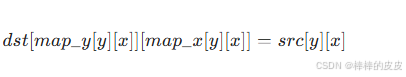
map_x:输出图像每个位置(x, y)对应的输入图像 x 坐标(形状与输入图像一致);map_y:输出图像每个位置(x, y)对应的输入图像 y 坐标(形状与输入图像一致);- 若映射坐标超出输入图像范围,可通过边界填充策略处理(如填充黑色、复制边界像素)。
2. 映射矩阵的构建逻辑
映射矩阵 map_x 和 map_y 是重映射的核心,需根据目标变换效果自定义:
- 基础变换(如镜像、旋转):可通过数学公式直接计算映射坐标;
- 复杂变换(如鱼眼、波浪):可通过三角函数、随机函数或外部数据定义映射关系;
- 映射矩阵的数据类型:必须为
np.float32(OpenCV 要求)。
3. OpenCV 重映射核心函数
OpenCV 通过 cv2.remap() 函数实现重映射,函数原型如下:
python
cv2.remap(src, map1, map2, interpolation, dst=None, borderMode=None, borderValue=None)参数说明
| 参数 | 含义 | 注意事项 |
|---|---|---|
src |
输入图像 | 单通道 / 多通道均可(灰度图 / 彩色图) |
map1 |
映射矩阵 1(x 坐标映射或联合映射) | 若为 x 坐标映射,需与 map2 配合;若为联合映射(如极坐标→笛卡尔坐标),map2 为标志位 |
map2 |
映射矩阵 2(y 坐标映射或标志位) | 与 map1 对应,常规重映射中为 y 坐标映射 |
interpolation |
插值算法 | 默认 cv2.INTER_LINEAR,常用 INTER_CUBIC(高质量)、INTER_NEAREST(快速) |
borderMode |
边界填充模式 | 默认 cv2.BORDER_CONSTANT(常数填充),可选 BORDER_REPLICATE(复制边界)等 |
borderValue |
边界填充值 | 仅 borderMode=BORDER_CONSTANT 有效,默认黑色(0),彩色图用 (b,g,r) 格式 |
关键说明
- 常规重映射场景中,
map1=map_x(x 坐标映射),map2=map_y(y 坐标映射); - 插值算法用于处理映射坐标为非整数的情况(如浮点数坐标),需根据效果和速度选择。
二、完整实现代码(多种场景)
1. 基础场景:实现常见简单变换
通过自定义映射矩阵,实现镜像、旋转、缩放等基础变换(验证重映射的灵活性):
python
import cv2
import numpy as np
import matplotlib.pyplot as plt

# 1. 读取图像
img = cv2.imread("lena.jpg")
if img is None:
    print("无法读取图像,请检查路径!")
    exit()
h, w = img.shape[:2]
img_rgb = cv2.cvtColor(img, cv2.COLOR_BGR2RGB)

# 2. 生成映射矩阵(初始化与图像同尺寸的float32矩阵)
map_x = np.zeros((h, w), dtype=np.float32)
map_y = np.zeros((h, w), dtype=np.float32)

# 3. 定义不同映射规则(按需注释/取消注释)
## 规则1:水平镜像(左右翻转,等价于 cv2.flip(img, 1))
for y in range(h):
    for x in range(w):
        map_x[y][x] = w - 1 - x  # x坐标反转
        map_y[y][x] = y          # y坐标不变

## 规则2:垂直镜像(上下翻转,等价于 cv2.flip(img, 0))
# for y in range(h):
#     for x in range(w):
#         map_x[y][x] = x
#         map_y[y][x] = h - 1 - y

## 规则3:缩放(缩小为原图1/2,居中显示)
# scale = 0.5
# new_w, new_h = int(w*scale), int(h*scale)
# map_x = np.zeros((h, w), dtype=np.float32)
# map_y = np.zeros((h, w), dtype=np.float32)
# for y in range(h):
#     for x in range(w):
#         map_x[y][x] = (x - w//2) * scale + w//2  # x方向缩放后居中
#         map_y[y][x] = (y - h//2) * scale + h//2  # y方向缩放后居中

## 规则4:90度旋转(顺时针,等价于 cv2.rotate(img, cv2.ROTATE_90_CLOCKWISE))
# map_x = np.zeros((h, w), dtype=np.float32)
# map_y = np.zeros((h, w), dtype=np.float32)
# for y in range(h):
#     for x in range(w):
#         map_x[y][x] = y
#         map_y[y][x] = w - 1 - x

# 4. 应用重映射
img_remap = cv2.remap(
    img, map_x, map_y,
    interpolation=cv2.INTER_LINEAR,
    borderValue=(255, 255, 255)  # 边界白色填充
)
img_remap_rgb = cv2.cvtColor(img_remap, cv2.COLOR_BGR2RGB)

# 5. 显示结果
plt.figure(figsize=(12, 6))
plt.subplot(1, 2, 1)
plt.imshow(img_rgb)
plt.title("Original Image")
plt.axis("off")
plt.subplot(1, 2, 2)
plt.imshow(img_remap_rgb)
plt.title("Remapped Image (Horizontal Mirror)")
plt.axis("off")
plt.tight_layout()
plt.show()
2. 创意场景:实现复杂特效(鱼眼、波浪、扭曲)
通过三角函数或随机函数定义映射规则,实现创意图像特效:
python
import cv2
import numpy as np
import matplotlib.pyplot as plt

# 1. 读取图像
img = cv2.imread("lena.jpg")
h, w = img.shape[:2]
img_rgb = cv2.cvtColor(img, cv2.COLOR_BGR2RGB)

# 2. 初始化映射矩阵
map_x = np.zeros((h, w), dtype=np.float32)
map_y = np.zeros((h, w), dtype=np.float32)

# 3. 定义特效映射规则(按需选择)
## 特效1:鱼眼效果(中心放大,边缘缩小)
cx, cy = w//2, h//2  # 图像中心
max_radius = min(cx, cy)  # 最大半径(避免超出图像)
for y in range(h):
    for x in range(w):
        # 计算当前点到中心的距离和角度
        dx = x - cx
        dy = y - cy
        radius = np.sqrt(dx**2 + dy**2)
        angle = np.arctan2(dy, dx)
        # 鱼眼畸变:距离中心越远,缩放比例越大(非线性缩放)
        distorted_radius = radius ** 0.8  # 指数越小,畸变越明显
        if distorted_radius > max_radius:
            distorted_radius = max_radius
        # 计算映射后的坐标
        map_x[y][x] = cx + distorted_radius * np.cos(angle)
        map_y[y][x] = cy + distorted_radius * np.sin(angle)

## 特效2:波浪效果(水平方向正弦扭曲)
# amplitude = 10  # 波浪振幅(扭曲程度)
# frequency = 20  # 波浪频率(密集程度)
# for y in range(h):
#     for x in range(w):
#         map_x[y][x] = x + amplitude * np.sin(y / frequency)  # x随y正弦变化
#         map_y[y][x] = y

## 特效3:随机扭曲(模拟抖动效果)
# np.random.seed(42)  # 固定随机种子,保证结果可复现
# distortion = 5  # 最大扭曲幅度
# for y in range(h):
#     for x in range(w):
#         map_x[y][x] = x + np.random.randint(-distortion, distortion+1)
#         map_y[y][x] = y + np.random.randint(-distortion, distortion+1)

# 4. 应用重映射(高质量插值)
img_remap = cv2.remap(
    img, map_x, map_y,
    interpolation=cv2.INTER_CUBIC,  # 复杂特效用双三次插值,减少锯齿
    borderValue=(255, 255, 255)
)
img_remap_rgb = cv2.cvtColor(img_remap, cv2.COLOR_BGR2RGB)

# 5. 显示结果
plt.figure(figsize=(12, 6))
plt.subplot(1, 2, 1)
plt.imshow(img_rgb)
plt.title("Original Image")
plt.axis("off")
plt.subplot(1, 2, 2)
plt.imshow(img_remap_rgb)
plt.title("Fisheye Effect (Remapping)")
plt.axis("off")
plt.tight_layout()
plt.show()
3. 实用场景:图像畸变校正(基于标定数据)
重映射的核心实用场景之一是镜头畸变校正:通过相机标定获得畸变参数后,生成校正映射矩阵,还原无畸变图像。
python
import cv2
import numpy as np
import matplotlib.pyplot as plt

def undistort_image(img, K, D):
    """
    基于相机标定参数的畸变校正(重映射实现)
    :param img: 畸变图像
    :param K: 相机内参矩阵(3×3)
    :param D: 畸变系数(1×5,[k1,k2,p1,p2,k3])
    :return: 校正后的无畸变图像
    """
    h, w = img.shape[:2]
    # 1. 生成无畸变的理想坐标(x,y)
    new_camera_matrix, roi = cv2.getOptimalNewCameraMatrix(K, D, (w, h), 1, (w, h))
    # 2. 计算畸变→无畸变的映射矩阵(map_x, map_y)
    map_x, map_y = cv2.initUndistortRectifyMap(
        K, D, None, new_camera_matrix, (w, h), cv2.CV_32FC1
    )
    # 3. 应用重映射
    undistorted_img = cv2.remap(
        img, map_x, map_y,
        interpolation=cv2.INTER_CUBIC,
        borderValue=(255, 255, 255)
    )
    # 裁剪无效区域(roi为有效区域坐标)
    x, y, w_roi, h_roi = roi
    undistorted_img = undistorted_img[y:y+h_roi, x:x+w_roi]
    return undistorted_img

# 1. 模拟相机标定参数(实际使用时需通过标定获得)
K = np.array([[500, 0, w//2],  # 内参矩阵:fx=500, fy=500, cx=w/2, cy=h/2
              [0, 500, h//2],
              [0, 0, 1]], dtype=np.float32)
D = np.array([[-0.2, 0.1, 0.001, 0.002, -0.05]], dtype=np.float32)  # 畸变系数(k1,k2,p1,p2,k3)

# 2. 读取畸变图像(或用普通图像模拟畸变)
img_distorted = cv2.imread("distorted.jpg")
if img_distorted is None:
    # 若无可畸变图像,用普通图像模拟畸变(可选)
    img = cv2.imread("lena.jpg")
    h, w = img.shape[:2]
    # 生成畸变映射矩阵(模拟径向畸变)
    map_x, map_y = cv2.initUndistortRectifyMap(K, D, None, K, (w, h), cv2.CV_32FC1)
    img_distorted = cv2.remap(img, map_x, map_y, cv2.INTER_LINEAR)

img_distorted_rgb = cv2.cvtColor(img_distorted, cv2.COLOR_BGR2RGB)

# 3. 畸变校正
img_undistorted = undistort_image(img_distorted, K, D)
img_undistorted_rgb = cv2.cvtColor(img_undistorted, cv2.COLOR_BGR2RGB)

# 4. 显示结果
plt.figure(figsize=(15, 8))
plt.subplot(1, 2, 1)
plt.imshow(img_distorted_rgb)
plt.title("Distorted Image")
plt.axis("off")
plt.subplot(1, 2, 2)
plt.imshow(img_undistorted_rgb)
plt.title("Undistorted Image (Remapping)")
plt.axis("off")
plt.tight_layout()
plt.show()

# 保存校正后的图像
cv2.imwrite("undistorted.jpg", img_undistorted)
print("畸变校正完成,已保存为 undistorted.jpg")
三、关键说明与应用场景
1. 重映射的核心优势
- 灵活性极高:无需遵循固定数学模型,可通过任意自定义规则实现变换;
- 精准控制:逐像素定义映射关系,可实现仿射 / 透视变换无法完成的复杂效果;
- 与标定结合:是相机畸变校正的核心实现方式,广泛用于计算机视觉系统。
2. 典型应用场景
- 图像特效制作:鱼眼、波浪、扭曲、抖动等创意效果(如游戏、影视后期);
- 相机畸变校正:去除镜头径向畸变、切向畸变,还原真实场景(如自动驾驶、机器人视觉);
- 自定义几何变换:实现仿射 / 透视变换无法覆盖的非线性变换(如不规则物体变形校正);
- 图像配准:多视角图像配准时,通过重映射统一像素坐标。
3. 与其他几何变换的区别
| 变换类型 | 核心特点 | 适用场景 |
|---|---|---|
| 重映射 | 自定义逐像素映射,无固定模型 | 复杂特效、畸变校正、自定义变形 |
| 仿射变换 | 保持平行性,2×3 矩阵,3 个点确定 | 平移、旋转、缩放、倾斜、简单校正 |
| 透视变换 | 不保持平行性,3×3 矩阵,4 个点确定 | 透视矫正、视角变换 |
四、注意事项
- 映射矩阵数据类型 :
map_x和map_y必须是np.float32类型,否则cv2.remap()会报错; - 坐标有效性 :若映射坐标超出输入图像范围,需通过
borderMode和borderValue处理边界(如复制边界或填充固定颜色); - 插值算法选择 :
- 简单变换(如镜像):用
cv2.INTER_LINEAR(速度快); - 复杂特效(如鱼眼):用
cv2.INTER_CUBIC(高质量,减少锯齿); - 实时场景:用
cv2.INTER_NEAREST(最快,牺牲少量质量);
- 简单变换(如镜像):用
- 性能优化 :
- 避免双重循环:大规模图像可通过
numpy向量运算替代for循环(如map_x = w - 1 - np.arange(w)[np.newaxis, :]),提升效率; - 预计算映射矩阵:若需重复应用同一变换,可预计算
map_x和map_y,避免重复计算;
- 避免双重循环:大规模图像可通过
- 相机标定参数 :畸变校正时,
K(内参矩阵)和D(畸变系数)需通过相机标定获得(如cv2.calibrateCamera()),模拟参数仅用于演示。
重映射是 OpenCV 中最灵活的几何变换方式,核心是掌握映射矩阵的构建逻辑。无论是创意特效还是实用的畸变校正,只要能定义像素的映射关系,就能通过 cv2.remap() 实现。在实际应用中,需平衡灵活性与性能,通过向量运算优化大规模图像的处理速度。