003 卷积神经网络（CNN）-- 原理到实践

目标

1. 理解卷积神经网络的核心思想和设计动机
2. 掌握卷积、池化等关键操作的工作原理
3. 使用PyTorch构建自己的CNN模型
4. 理解CNN在图像分类、目标检测等任务中的应用
5. 调试和优化CNN模型

---

第一部分：为什么需要卷积神经网络？

1.1 传统神经网络处理图像的局限性

让我们先思考一个问题：如果使用之前学过的全连接神经网络处理一张图片，会有什么问题？

import torch
import numpy as np

# 假设有一张 224x224 的彩色图片
image_height = 224
image_width = 224
channels = 3  # RGB三通道

# 将图片展平后输入全连接网络
flattened_size = image_height * image_width * channels  # 224 * 224 * 3 = 150,528
print(f"一张224x224的彩色图片展平后：{flattened_size:,} 个输入特征")

# 假设第一个隐藏层有512个神经元
hidden_units = 512

# 计算第一层的参数量
parameters = (flattened_size + 1) * hidden_units  # +1 是偏置项
print(f"第一层参数数量：{parameters:,}")

# 参数量太大导致的问题：
print("\n⚠️ 全连接网络处理图像的问题：")
print("1. 参数量爆炸：150,528 × 512 = 77,000,000+ 参数")
print("2. 计算效率低：需要大量矩阵乘法")
print("3. 容易过拟合：参数太多，数据不足")
print("4. 忽略了空间结构：像素之间的位置关系丢失")

输出结果：

一张224x224的彩色图片展平后：150,528 个输入特征
第一层参数数量：77,115,392

⚠️ 全连接网络处理图像的问题：
1. 参数量爆炸：150,528 × 512 = 77,000,000+ 参数
2. 计算效率低：需要大量矩阵乘法
3. 容易过拟合：参数太多，数据不足
4. 忽略了空间结构：像素之间的位置关系丢失

1.2 CNN的三大核心思想

卷积神经网络通过三个关键思想解决了上述问题：

1. 局部连接（Local Connectivity）

不是每个神经元都连接到所有输入，只连接输入的一小部分区域

2. 权重共享（Weight Sharing）

同一个滤波器（卷积核）在整个图像上滑动使用，大大减少参数

3. 空间下采样（Spatial Subsampling）

通过池化操作减少特征图尺寸，保留重要信息

---

第二部分：CNN核心组件详解

2.1 卷积操作（Convolution）

直观理解：特征检测器

想象你有一张照片，想找出其中的边缘、纹理等特征。卷积操作就像用一个小窗口（滤波器） 在图片上滑动，检测特定的模式。

import matplotlib.pyplot as plt
import numpy as np

# 创建一个简单的6x6图像（模拟边缘）
image = np.array([
    [1, 1, 1, 0, 0, 0],
    [1, 1, 1, 0, 0, 0],
    [1, 1, 1, 0, 0, 0],
    [1, 1, 1, 0, 0, 0],
    [1, 1, 1, 0, 0, 0],
    [1, 1, 1, 0, 0, 0]
])

# 创建两个不同的卷积核（滤波器）
vertical_edge_kernel = np.array([  # 垂直边缘检测
    [1, 0, -1],
    [1, 0, -1],
    [1, 0, -1]
])

horizontal_edge_kernel = np.array([  # 水平边缘检测
    [1, 1, 1],
    [0, 0, 0],
    [-1, -1, -1]
])

print("原始图像（6x6，左侧亮，右侧暗）：")
print(image)
print("\n垂直边缘检测核（3x3）：")
print(vertical_edge_kernel)
print("\n水平边缘检测核（3x3）：")
print(horizontal_edge_kernel)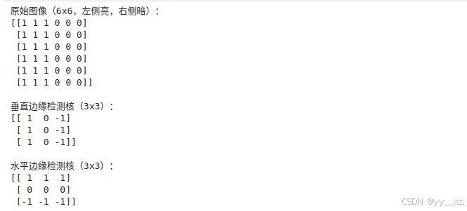

卷积运算的数学过程

def manual_convolution(image, kernel):
    """手动实现卷积操作"""
    img_h, img_w = image.shape
    kernel_h, kernel_w = kernel.shape
    
    # 输出特征图尺寸
    output_h = img_h - kernel_h + 1
    output_w = img_w - kernel_w + 1
    
    output = np.zeros((output_h, output_w))
    
    # 滑动窗口计算卷积
    for i in range(output_h):
        for j in range(output_w):
            # 提取图像块
            patch = image[i:i+kernel_h, j:j+kernel_w]
            # 逐元素相乘并求和
            output[i, j] = np.sum(patch * kernel)
    
    return output

# 应用卷积
vertical_edges = manual_convolution(image, vertical_edge_kernel)
horizontal_edges = manual_convolution(image, horizontal_edge_kernel)

print("\n卷积结果 - 垂直边缘检测：")
print(vertical_edges)
print("\n卷积结果 - 水平边缘检测：")
print(horizontal_edges)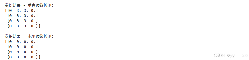

可视化卷积过程：

def visualize_convolution(image, kernel, result):
    """可视化卷积过程"""
    fig, axes = plt.subplots(1, 3, figsize=(12, 4))
    
    # 原始图像
    axes[0].imshow(image, cmap='gray', vmin=0, vmax=1)
    axes[0].set_title('原始图像')
    axes[0].set_xticks(range(image.shape[1]))
    axes[0].set_yticks(range(image.shape[0]))
    axes[0].grid(True, alpha=0.3)
    
    # 卷积核
    axes[1].imshow(kernel, cmap='coolwarm', vmin=-1, vmax=1)
    axes[1].set_title('卷积核（滤波器）')
    axes[1].set_xticks(range(kernel.shape[1]))
    axes[1].set_yticks(range(kernel.shape[0]))
    
    # 添加核值标注
    for i in range(kernel.shape[0]):
        for j in range(kernel.shape[1]):
            axes[1].text(j, i, f'{kernel[i, j]}', 
                        ha='center', va='center', 
                        color='white' if abs(kernel[i, j]) > 0.5 else 'black')
    
    # 卷积结果
    axes[2].imshow(result, cmap='gray')
    axes[2].set_title('卷积结果（特征图）')
    axes[2].set_xticks(range(result.shape[1]))
    axes[2].set_yticks(range(result.shape[0]))
    axes[2].grid(True, alpha=0.3)
    
    # 添加结果值标注
    for i in range(result.shape[0]):
        for j in range(result.shape[1]):
            axes[2].text(j, i, f'{result[i, j]:.0f}', 
                        ha='center', va='center', 
                        color='white' if abs(result[i, j]) > 2 else 'black')
    
    plt.tight_layout()
    plt.show()

# 可视化
print("\n垂直边缘检测过程：")
visualize_convolution(image, vertical_edge_kernel, vertical_edges)

print("\n水平边缘检测过程：")
visualize_convolution(image, horizontal_edge_kernel, horizontal_edges)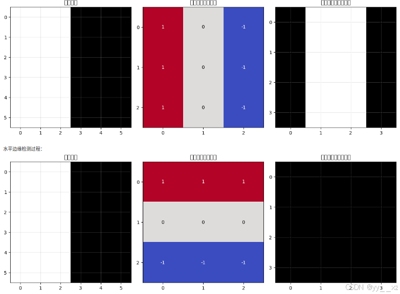

卷积的重要概念

# 演示CNN中的关键参数
def explain_convolution_parameters():
    print("="*60)
    print("卷积操作的关键参数详解")
    print("="*60)
    
    print("\n1. 卷积核大小（Kernel Size）:")
    print("   - 常见大小：3×3, 5×5, 7×7")
    print("   - 小的核（3×3）：感受野小，捕获局部特征")
    print("   - 大的核（7×7）：感受野大，捕获全局特征")
    
    print("\n2. 步幅（Stride）:")
    print("   - 卷积核每次滑动的距离")
    print("   - stride=1：每次移动1像素，输出尺寸大")
    print("   - stride=2：每次移动2像素，输出尺寸减半")
    
    print("\n3. 填充（Padding）:")
    print("   - 在图像边缘添加0值像素")
    print("   - 'same' padding：输出尺寸与输入相同")
    print("   - 'valid' padding：不填充，输出尺寸变小")
    
    print("\n4. 通道数（Channels）:")
    print("   - 输入通道：彩色图像为3（RGB），灰度图像为1")
    print("   - 输出通道：卷积核的数量，每个核学习不同特征")
    
    print("\n5. 特征图计算公式:")
    print("   - 输出高度 = (输入高度 + 2×填充 - 核高度) / 步幅 + 1")
    print("   - 输出宽度 = (输入宽度 + 2×填充 - 核宽度) / 步幅 + 1")

explain_convolution_parameters()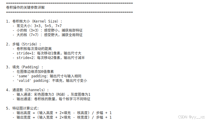

2.2 激活函数（Activation Function）

卷积后通常要加激活函数，引入非线性。

import torch
import torch.nn.functional as F

# 演示不同的激活函数
def demo_activation_functions():
    # 创建一些数据
    x = torch.linspace(-5, 5, 100)
    
    # 计算不同激活函数的输出
    relu = F.relu(x)
    sigmoid = torch.sigmoid(x)
    tanh = torch.tanh(x)
    leaky_relu = F.leaky_relu(x, negative_slope=0.1)
    
    # 可视化
    plt.figure(figsize=(12, 8))
    
    activations = [
        ('ReLU', relu, 'red'),
        ('Sigmoid', sigmoid, 'blue'),
        ('Tanh', tanh, 'green'),
        ('Leaky ReLU (α=0.1)', leaky_relu, 'orange')
    ]
    
    for i, (name, activation, color) in enumerate(activations, 1):
        plt.subplot(2, 2, i)
        plt.plot(x.numpy(), activation.numpy(), color=color, linewidth=3)
        plt.title(name)
        plt.xlabel('输入')
        plt.ylabel('输出')
        plt.grid(True, alpha=0.3)
        plt.axhline(y=0, color='black', linestyle='-', alpha=0.3)
        plt.axvline(x=0, color='black', linestyle='-', alpha=0.3)
    
    plt.suptitle('常用激活函数对比', fontsize=16)
    plt.tight_layout()
    plt.show()
    
    print("\nCNN中常用的激活函数：")
    print("1. ReLU（最常用）:")
    print("   - 优点：计算简单，缓解梯度消失")
    print("   - 缺点：负区间梯度为0（神经元'死亡'）")
    
    print("\n2. Leaky ReLU:")
    print("   - 优点：负区间有小的梯度，缓解神经元死亡")
    
    print("\n3. Sigmoid（用于输出层）:")
    print("   - 优点：输出在0-1之间，适合概率")
    print("   - 缺点：容易梯度消失")

demo_activation_functions()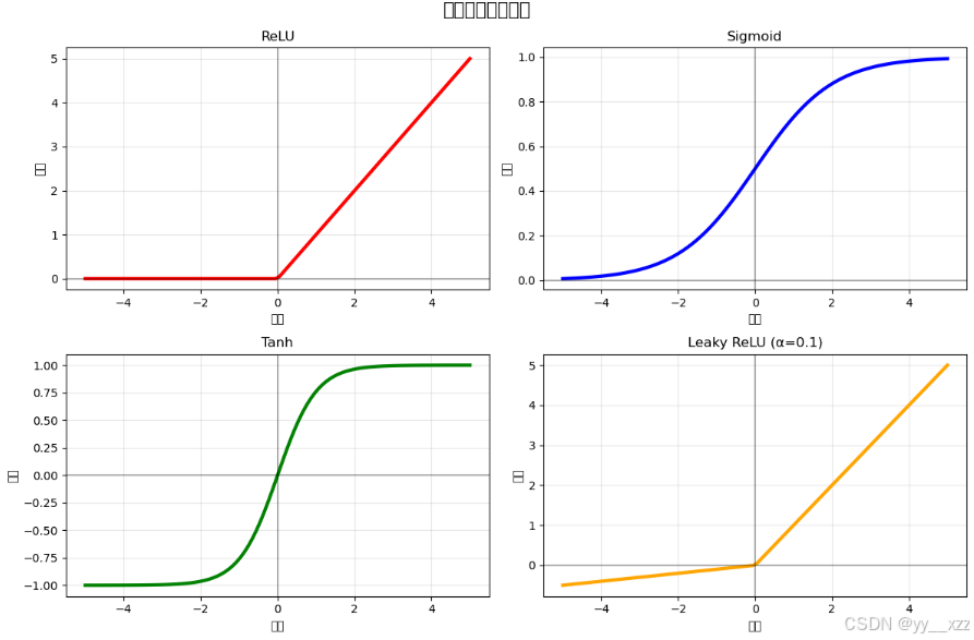

2.3 池化操作（Pooling）

池化的目的是降维 和增加平移不变性。

def demo_pooling_operations():
    # 创建一个4x4的特征图
    feature_map = np.array([
        [1, 2, 5, 3],
        [4, 8, 6, 2],
        [7, 3, 9, 1],
        [2, 5, 4, 6]
    ])
    
    print("原始特征图（4x4）：")
    print(feature_map)
    
    # 最大池化（2x2，步幅2）
    def max_pooling_2d(matrix, pool_size=2, stride=2):
        h, w = matrix.shape
        output_h = (h - pool_size) // stride + 1
        output_w = (w - pool_size) // stride + 1
        
        output = np.zeros((output_h, output_w))
        
        for i in range(0, h - pool_size + 1, stride):
            for j in range(0, w - pool_size + 1, stride):
                patch = matrix[i:i+pool_size, j:j+pool_size]
                output[i//stride, j//stride] = np.max(patch)
        
        return output
    
    # 平均池化（2x2，步幅2）
    def avg_pooling_2d(matrix, pool_size=2, stride=2):
        h, w = matrix.shape
        output_h = (h - pool_size) // stride + 1
        output_w = (w - pool_size) // stride + 1
        
        output = np.zeros((output_h, output_w))
        
        for i in range(0, h - pool_size + 1, stride):
            for j in range(0, w - pool_size + 1, stride):
                patch = matrix[i:i+pool_size, j:j+pool_size]
                output[i//stride, j//stride] = np.mean(patch)
        
        return output
    
    max_pool_result = max_pooling_2d(feature_map)
    avg_pool_result = avg_pooling_2d(feature_map)
    
    print("\n最大池化结果（2x2）：")
    print(max_pool_result)
    
    print("\n平均池化结果（2x2）：")
    print(avg_pool_result)
    
    # 可视化
    fig, axes = plt.subplots(1, 3, figsize=(12, 4))
    
    # 原始特征图
    im1 = axes[0].imshow(feature_map, cmap='viridis')
    axes[0].set_title('原始特征图 (4x4)')
    axes[0].set_xticks(range(4))
    axes[0].set_yticks(range(4))
    plt.colorbar(im1, ax=axes[0], fraction=0.046, pad=0.04)
    
    # 最大池化
    im2 = axes[1].imshow(max_pool_result, cmap='viridis')
    axes[1].set_title('最大池化结果 (2x2)')
    axes[1].set_xticks(range(2))
    axes[1].set_yticks(range(2))
    plt.colorbar(im2, ax=axes[1], fraction=0.046, pad=0.04)
    
    # 平均池化
    im3 = axes[2].imshow(avg_pool_result, cmap='viridis')
    axes[2].set_title('平均池化结果 (2x2)')
    axes[2].set_xticks(range(2))
    axes[2].set_yticks(range(2))
    plt.colorbar(im3, ax=axes[2], fraction=0.046, pad=0.04)
    
    plt.tight_layout()
    plt.show()
    
    print("\n池化操作的作用：")
    print("1. 降维：减少计算量和参数")
    print("2. 平移不变性：物体轻微移动不影响识别")
    print("3. 防止过拟合：减少空间信息，增加鲁棒性")
    print("4. 扩大感受野：池化后每个神经元看到更大区域")
    
    print("\n最大池化 vs 平均池化：")
    print("最大池化：保留最显著特征，常用于图像")
    print("平均池化：保留整体信息，对噪声更鲁棒")

demo_pooling_operations()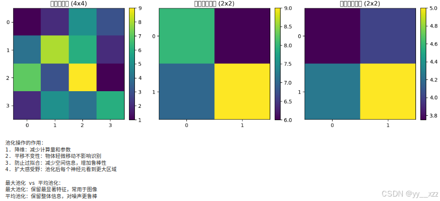

2.4 全连接层（Fully Connected Layer）

在CNN的最后，通常会有1-3个全连接层，用于最终的分类或回归。

def explain_fc_layers():
    print("="*60)
    print("CNN中的全连接层")
    print("="*60)
    
    print("\n全连接层的作用：")
    print("1. 整合特征：将卷积提取的局部特征组合成全局特征")
    print("2. 进行分类：输出每个类别的概率")
    print("3. 进行回归：输出预测值")
    
    print("\n典型CNN架构中的全连接层：")
    print("输入 → [卷积层 → 激活 → 池化] × N → 展平 → 全连接层 → 输出")
    
    print("\n展平操作（Flatten）：")
    print("将多维特征图转换为一维向量")
    print("例如：64个7×7的特征图 → 展平为 64×7×7 = 3136维向量")
    
    print("\n现代CNN的趋势：")
    print("1. 减少全连接层参数（使用全局平均池化）")
    print("2. 增加Dropout防止过拟合")
    print("3. 使用批归一化加速训练")

explain_fc_layers()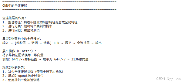

---

第三部分：经典CNN架构分析

3.1 LeNet-5（1998年） - CNN的开山之作

import torch.nn as nn

class LeNet5(nn.Module):
    """LeNet-5 - 最早的CNN架构，用于手写数字识别"""
    
    def __init__(self, num_classes=10):
        super(LeNet5, self).__init__()
        
        # 特征提取部分
        self.features = nn.Sequential(
            # 卷积层1: 输入1通道，输出6通道，5x5卷积核
            nn.Conv2d(in_channels=1, out_channels=6, kernel_size=5),
            nn.Tanh(),  # 原始LeNet使用Tanh
            # 平均池化层: 2x2池化
            nn.AvgPool2d(kernel_size=2, stride=2),
            
            # 卷积层2: 输入6通道，输出16通道，5x5卷积核
            nn.Conv2d(in_channels=6, out_channels=16, kernel_size=5),
            nn.Tanh(),
            nn.AvgPool2d(kernel_size=2, stride=2),
        )
        
        # 分类部分
        self.classifier = nn.Sequential(
            # 展平后输入: 16*4*4 = 256（假设输入32x32）
            nn.Linear(16 * 4 * 4, 120),
            nn.Tanh(),
            nn.Linear(120, 84),
            nn.Tanh(),
            nn.Linear(84, num_classes),
        )
    
    def forward(self, x):
        x = self.features(x)
        x = x.view(x.size(0), -1)  # 展平
        x = self.classifier(x)
        return x

# 创建LeNet实例
lenet = LeNet5()
print("LeNet-5 架构分析：")
print(lenet)
print("\n参数量分析：")
total_params = sum(p.numel() for p in lenet.parameters())
print(f"总参数量：{total_params:,}")
print(f"可训练参数：{sum(p.numel() for p in lenet.parameters() if p.requires_grad):,}")

print("\nLeNet-5的历史意义：")
print("1. 首次成功应用CNN于实际任务（手写数字识别）")
print("2. 确立了CNN的基本结构：卷积 → 池化 → 全连接")
print("3. 启发了后续所有CNN架构")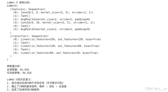

3.2 AlexNet（2012年） - 深度学习复兴的标志

class AlexNet(nn.Module):
    """AlexNet - 2012年ImageNet冠军，深度学习复兴的标志"""
    
    def __init__(self, num_classes=1000):
        super(AlexNet, self).__init__()
        
        self.features = nn.Sequential(
            # 第一层: 大卷积核
            nn.Conv2d(3, 64, kernel_size=11, stride=4, padding=2),
            nn.ReLU(inplace=True),
            nn.MaxPool2d(kernel_size=3, stride=2),
            
            # 第二层
            nn.Conv2d(64, 192, kernel_size=5, padding=2),
            nn.ReLU(inplace=True),
            nn.MaxPool2d(kernel_size=3, stride=2),
            
            # 第三层
            nn.Conv2d(192, 384, kernel_size=3, padding=1),
            nn.ReLU(inplace=True),
            
            # 第四层
            nn.Conv2d(384, 256, kernel_size=3, padding=1),
            nn.ReLU(inplace=True),
            
            # 第五层
            nn.Conv2d(256, 256, kernel_size=3, padding=1),
            nn.ReLU(inplace=True),
            nn.MaxPool2d(kernel_size=3, stride=2),
        )
        
        self.avgpool = nn.AdaptiveAvgPool2d((6, 6))
        
        self.classifier = nn.Sequential(
            nn.Dropout(p=0.5),  # AlexNet首次使用了Dropout
            nn.Linear(256 * 6 * 6, 4096),
            nn.ReLU(inplace=True),
            nn.Dropout(p=0.5),
            nn.Linear(4096, 4096),
            nn.ReLU(inplace=True),
            nn.Linear(4096, num_classes),
        )
    
    def forward(self, x):
        x = self.features(x)
        x = self.avgpool(x)
        x = x.view(x.size(0), -1)
        x = self.classifier(x)
        return x

# AlexNet的创新点
print("="*60)
print("AlexNet的创新点：")
print("="*60)
print("1. 使用ReLU激活函数：缓解梯度消失，加速训练")
print("2. 使用Dropout：防止过拟合")
print("3. 数据增强：增加训练数据多样性")
print("4. 多GPU训练：当时在2个GPU上并行训练")
print("5. 局部响应归一化（LRN）：增加局部竞争")
print("6. 重叠池化：提高精度，缓解过拟合")

alexnet = AlexNet()
total_params = sum(p.numel() for p in alexnet.parameters())
print(f"\nAlexNet参数量：{total_params:,}（约6000万）")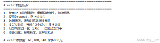

3.3 现代CNN架构趋势

def explain_cnn_evolution():
    print("\n" + "="*60)
    print("CNN架构演化趋势")
    print("="*60)
    
    print("\n1. 从大卷积核到小卷积核：")
    print("   LeNet: 5×5, 5×5")
    print("   AlexNet: 11×11, 5×5, 3×3")
    print("   VGG: 全部使用3×3")
    print("   趋势：小卷积核减少参数，增加非线性")
    
    print("\n2. 从浅到深：")
    print("   LeNet: 2个卷积层")
    print("   AlexNet: 5个卷积层")
    print("   VGG-16: 13个卷积层")
    print("   ResNet: 最多152个卷积层")
    print("   趋势：更深的网络学习更复杂的特征")
    
    print("\n3. 从复杂到简洁：")
    print("   AlexNet: 复杂结构，定制化设计")
    print("   VGG: 模块化设计，规则结构")
    print("   ResNet: 残差连接，解决梯度消失")
    
    print("\n4. 全连接层的演变：")
    print("   早期：多个全连接层（AlexNet有3个）")
    print("   现代：减少或不用全连接层")
    print("   替代：全局平均池化（Global Average Pooling）")

explain_cnn_evolution()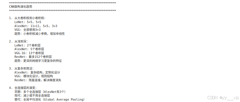

---

第四部分：PyTorch实现CNN实战

4.1 使用CNN进行图像分类（CIFAR-10）

import torch
import torch.nn as nn
import torch.optim as optim
import torchvision
import torchvision.transforms as transforms
from torch.utils.data import DataLoader
import matplotlib.pyplot as plt

class SimpleCNN(nn.Module):
    """一个简单的CNN，用于CIFAR-10分类"""
    
    def __init__(self, num_classes=10):
        super(SimpleCNN, self).__init__()
        
        # 卷积块1
        self.conv_block1 = nn.Sequential(
            nn.Conv2d(3, 32, kernel_size=3, padding=1),  # 32x32x3 → 32x32x32
            nn.BatchNorm2d(32),
            nn.ReLU(inplace=True),
            nn.Conv2d(32, 32, kernel_size=3, padding=1),  # 32x32x32 → 32x32x32
            nn.BatchNorm2d(32),
            nn.ReLU(inplace=True),
            nn.MaxPool2d(kernel_size=2, stride=2),  # 32x32x32 → 16x16x32
            nn.Dropout2d(0.2)
        )
        
        # 卷积块2
        self.conv_block2 = nn.Sequential(
            nn.Conv2d(32, 64, kernel_size=3, padding=1),  # 16x16x32 → 16x16x64
            nn.BatchNorm2d(64),
            nn.ReLU(inplace=True),
            nn.Conv2d(64, 64, kernel_size=3, padding=1),  # 16x16x64 → 16x16x64
            nn.BatchNorm2d(64),
            nn.ReLU(inplace=True),
            nn.MaxPool2d(kernel_size=2, stride=2),  # 16x16x64 → 8x8x64
            nn.Dropout2d(0.3)
        )
        
        # 卷积块3
        self.conv_block3 = nn.Sequential(
            nn.Conv2d(64, 128, kernel_size=3, padding=1),  # 8x8x64 → 8x8x128
            nn.BatchNorm2d(128),
            nn.ReLU(inplace=True),
            nn.Conv2d(128, 128, kernel_size=3, padding=1),  # 8x8x128 → 8x8x128
            nn.BatchNorm2d(128),
            nn.ReLU(inplace=True),
            nn.MaxPool2d(kernel_size=2, stride=2),  # 8x8x128 → 4x4x128
            nn.Dropout2d(0.4)
        )
        
        # 分类器
        self.classifier = nn.Sequential(
            nn.Flatten(),  # 4x4x128 = 2048
            nn.Linear(128 * 4 * 4, 512),
            nn.BatchNorm1d(512),
            nn.ReLU(inplace=True),
            nn.Dropout(0.5),
            nn.Linear(512, num_classes)
        )
    
    def forward(self, x):
        x = self.conv_block1(x)
        x = self.conv_block2(x)
        x = self.conv_block3(x)
        x = self.classifier(x)
        return x

def train_cifar10():
    """训练CNN进行CIFAR-10分类"""
    
    # 数据预处理
    transform = transforms.Compose([
        transforms.RandomHorizontalFlip(),  # 数据增强
        transforms.RandomCrop(32, padding=4),
        transforms.ToTensor(),
        transforms.Normalize((0.4914, 0.4822, 0.4465),  # CIFAR-10的均值和标准差
                            (0.2470, 0.2435, 0.2616))
    ])
    
    # 加载数据集
    train_dataset = torchvision.datasets.CIFAR10(
        root='./data', train=True, download=True, transform=transform
    )
    
    test_dataset = torchvision.datasets.CIFAR10(
        root='./data', train=False, download=True, transform=transforms.ToTensor()
    )
    
    # 创建数据加载器
    train_loader = DataLoader(train_dataset, batch_size=128, shuffle=True, num_workers=2)
    test_loader = DataLoader(test_dataset, batch_size=100, shuffle=False, num_workers=2)
    
    # 创建模型
    model = SimpleCNN(num_classes=10)
    device = torch.device('cuda' if torch.cuda.is_available() else 'cpu')
    model = model.to(device)
    
    print(f"使用设备: {device}")
    print(f"模型参数量: {sum(p.numel() for p in model.parameters()):,}")
    
    # 定义损失函数和优化器
    criterion = nn.CrossEntropyLoss()
    optimizer = optim.Adam(model.parameters(), lr=0.001)
    scheduler = optim.lr_scheduler.ReduceLROnPlateau(optimizer, mode='min', patience=5)
    
    # 训练循环
    num_epochs = 30
    train_losses, test_accuracies = [], []
    
    for epoch in range(num_epochs):
        # 训练阶段
        model.train()
        running_loss = 0.0
        
        for batch_idx, (inputs, targets) in enumerate(train_loader):
            inputs, targets = inputs.to(device), targets.to(device)
            
            # 前向传播
            outputs = model(inputs)
            loss = criterion(outputs, targets)
            
            # 反向传播
            optimizer.zero_grad()
            loss.backward()
            optimizer.step()
            
            running_loss += loss.item()
            
            if batch_idx % 100 == 0:
                print(f'Epoch [{epoch+1}/{num_epochs}] | '
                      f'Batch [{batch_idx+1}/{len(train_loader)}] | '
                      f'Loss: {loss.item():.4f}')
        
        avg_loss = running_loss / len(train_loader)
        train_losses.append(avg_loss)
        
        # 测试阶段
        model.eval()
        correct = 0
        total = 0
        
        with torch.no_grad():
            for inputs, targets in test_loader:
                inputs, targets = inputs.to(device), targets.to(device)
                outputs = model(inputs)
                _, predicted = outputs.max(1)
                total += targets.size(0)
                correct += predicted.eq(targets).sum().item()
        
        accuracy = 100. * correct / total
        test_accuracies.append(accuracy)
        
        # 学习率调整
        scheduler.step(avg_loss)
        
        print(f'Epoch [{epoch+1}/{num_epochs}] | '
              f'Train Loss: {avg_loss:.4f} | '
              f'Test Accuracy: {accuracy:.2f}% | '
              f'LR: {optimizer.param_groups[0]["lr"]:.6f}')
    
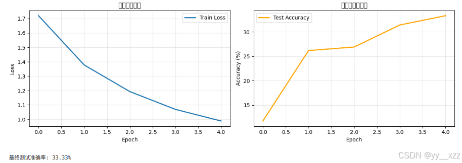
    # 可视化训练过程
    plt.figure(figsize=(12, 4))
    
    plt.subplot(1, 2, 1)
    plt.plot(train_losses, label='Train Loss', linewidth=2)
    plt.xlabel('Epoch')
    plt.ylabel('Loss')
    plt.title('训练损失曲线')
    plt.legend()
    plt.grid(True, alpha=0.3)
    
    plt.subplot(1, 2, 2)
    plt.plot(test_accuracies, label='Test Accuracy', linewidth=2, color='orange')
    plt.xlabel('Epoch')
    plt.ylabel('Accuracy (%)')
    plt.title('测试准确率曲线')
    plt.legend()
    plt.grid(True, alpha=0.3)
    
    plt.tight_layout()
    plt.show()
    
    print(f"\n最终测试准确率: {test_accuracies[-1]:.2f}%")
    
    return model

# 注意：实际运行会耗时较长，建议在GPU上运行
model = train_cifar10()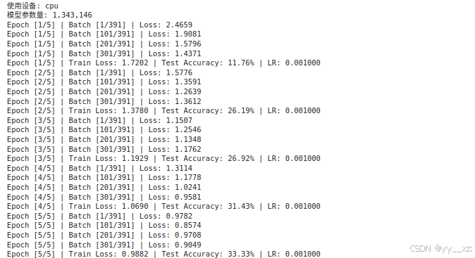

4.2 CNN特征可视化

def visualize_cnn_features(model, image):
    """可视化CNN各层的特征图"""
    
    # 获取模型的卷积层
    conv_layers = []
    for layer in model.modules():
        if isinstance(layer, nn.Conv2d):
            conv_layers.append(layer)
    
    print(f"模型有 {len(conv_layers)} 个卷积层")
    
    # 创建钩子函数来获取中间特征
    features = []
    def hook_fn(module, input, output):
        features.append(output.detach())
    
    # 注册钩子
    hooks = []
    for layer in conv_layers[:4]:  # 只可视化前4层
        hooks.append(layer.register_forward_hook(hook_fn))
    
    # 前向传播
    model.eval()
    with torch.no_grad():
        _ = model(image.unsqueeze(0))  # 添加batch维度
    
    # 移除钩子
    for hook in hooks:
        hook.remove()
    
    # 可视化特征图
    num_layers = len(features)
    fig, axes = plt.subplots(num_layers, 8, figsize=(16, num_layers*2))
    
    for i, feature in enumerate(features):
        # 选择前8个通道
        num_channels = min(8, feature.size(1))
        
        for j in range(num_channels):
            if num_layers == 1:
                ax = axes[j]
            else:
                ax = axes[i, j]
            
            channel_data = feature[0, j].cpu().numpy()
            
            # 归一化到0-1以便显示
            if channel_data.max() > channel_data.min():
                channel_data = (channel_data - channel_data.min()) / (channel_data.max() - channel_data.min())
            
            ax.imshow(channel_data, cmap='viridis')
            ax.set_xticks([])
            ax.set_yticks([])
            
            if j == 0:
                ax.set_ylabel(f'Conv{i+1}', fontsize=12)
    
    plt.suptitle('CNN各层特征图可视化', fontsize=16)
    plt.tight_layout()
    plt.show()

# 示例：可视化特征图（需要先有训练好的模型和图片）
# visualize_cnn_features(model, sample_image)

---

第五部分：CNN进阶话题

5.1 1x1卷积的作用

def explain_1x1_convolution():
    print("="*60)
    print("1×1卷积的神奇作用")
    print("="*60)
    
    print("\n1. 通道维度变换（降维/升维）：")
    print("   输入：H×W×C_in → 输出：H×W×C_out")
    print("   例如：256通道 → 64通道（降维）")
    print("   例如：64通道 → 256通道（升维）")
    
    print("\n2. 增加非线性：")
    print("   1×1卷积 + 激活函数 = 非线性变换")
    print("   可以组合通道间的信息")
    
    print("\n3. 减少计算量：")
    print("   在Inception网络和ResNet中广泛使用")
    print("   先用1×1卷积降维，再用3×3卷积")
    
    print("\n4. 示例代码：")
    
    # 演示1x1卷积
    input_channels = 256
    output_channels = 64
    
    # 传统3x3卷积
    conv3x3 = nn.Conv2d(input_channels, output_channels, kernel_size=3, padding=1)
    params_3x3 = sum(p.numel() for p in conv3x3.parameters())
    
    # 使用1x1卷积降维后再用3x3
    conv1x1_reduce = nn.Conv2d(input_channels, 64, kernel_size=1)  # 降到64通道
    conv3x3_small = nn.Conv2d(64, output_channels, kernel_size=3, padding=1)
    params_1x1_3x3 = sum(p.numel() for p in conv1x1_reduce.parameters()) + \
                     sum(p.numel() for p in conv3x3_small.parameters())
    
    print(f"   直接3×3卷积参数量：{params_3x3:,}")
    print(f"   1×1降维+3×3卷积参数量：{params_1x1_3x3:,}")
    print(f"   参数减少：{(1 - params_1x1_3x3/params_3x3)*100:.1f}%")

explain_1x1_convolution()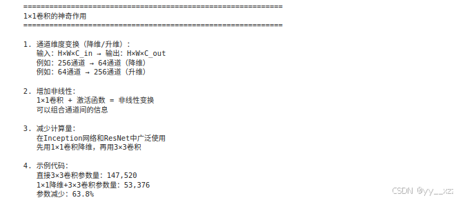

5.2 感受野计算

def calculate_receptive_field():
    """计算CNN的感受野"""
    
    print("="*60)
    print("感受野（Receptive Field）计算")
    print("="*60)
    
    print("\n感受野定义：")
    print("输出特征图上的一个像素，对应输入图像上的区域大小")
    
    print("\n计算规则：")
    print("1. 第一层感受野 = 卷积核大小")
    print("2. 后续每层：感受野 = 上一层的感受野 + (卷积核大小-1) × 前面所有层的步幅乘积")
    
    print("\n示例：VGG-16的感受野计算")
    
    # VGG-16的架构
    layers = [
        ('conv3', 3, 1),  # 卷积核大小，步幅
        ('conv3', 3, 1),
        ('pool2', 2, 2),  # 池化大小，步幅
        ('conv3', 3, 1),
        ('conv3', 3, 1),
        ('pool2', 2, 2),
        ('conv3', 3, 1),
        ('conv3', 3, 1),
        ('conv3', 3, 1),
        ('pool2', 2, 2),
        ('conv3', 3, 1),
        ('conv3', 3, 1),
        ('conv3', 3, 1),
        ('pool2', 2, 2),
        ('conv3', 3, 1),
        ('conv3', 3, 1),
        ('conv3', 3, 1),
        ('pool2', 2, 2),
    ]
    
    receptive_field = 1
    total_stride = 1
    
    print("\n层-by-层感受野计算：")
    for i, (layer_name, kernel_size, stride) in enumerate(layers):
        if 'conv' in layer_name:
            receptive_field = receptive_field + (kernel_size - 1) * total_stride
        elif 'pool' in layer_name:
            receptive_field = receptive_field + (kernel_size - 1) * total_stride
        
        total_stride *= stride
        
        print(f"第{i+1:2d}层 {layer_name:6s} | "
              f"感受野: {receptive_field:3d} | "
              f"累积步幅: {total_stride}")
    
    print(f"\n最终感受野: {receptive_field}")
    print("这意味着输出层的一个神经元能看到输入图像上{receptive_field}×{receptive_field}的区域")

calculate_receptive_field()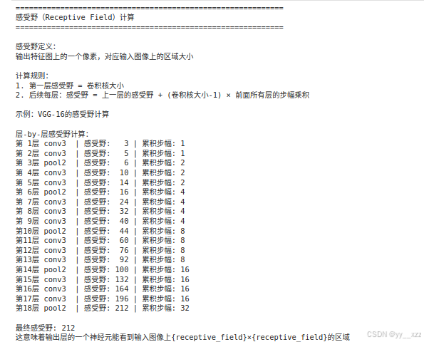

5.3 批归一化（Batch Normalization）

def explain_batch_norm():
    print("\n" + "="*60)
    print("批归一化（Batch Normalization）")
    print("="*60)
    
    print("\n问题：内部协变量偏移（Internal Covariate Shift）")
    print("网络每层的输入分布会随着训练而变化")
    print("导致训练困难，需要小心调整学习率")
    
    print("\n批归一化的解决方案：")
    print("1. 对每个batch的数据进行标准化")
    print("2. 学习两个参数：缩放γ和平移β")
    print("3. 公式：BN(x) = γ × (x - μ)/σ + β")
    
    print("\n批归一化的好处：")
    print("1. 允许使用更大的学习率")
    print("2. 减少对初始化的依赖")
    print("3. 有轻微的正则化效果")
    print("4. 加速训练收敛")
    
    print("\n在CNN中的使用位置：")
    print("卷积层后、激活函数前（最常用）")
    print("Conv → BN → ReLU → Pooling")
    
    print("\n代码示例：")
    print("""
class ConvBlock(nn.Module):
    def __init__(self, in_channels, out_channels):
        super().__init__()
        self.conv = nn.Conv2d(in_channels, out_channels, 3, padding=1)
        self.bn = nn.BatchNorm2d(out_channels)  # 批归一化
        self.relu = nn.ReLU(inplace=True)
        
    def forward(self, x):
        x = self.conv(x)
        x = self.bn(x)    # 批归一化
        x = self.relu(x)  # 激活函数
        return x
    """)

explain_batch_norm()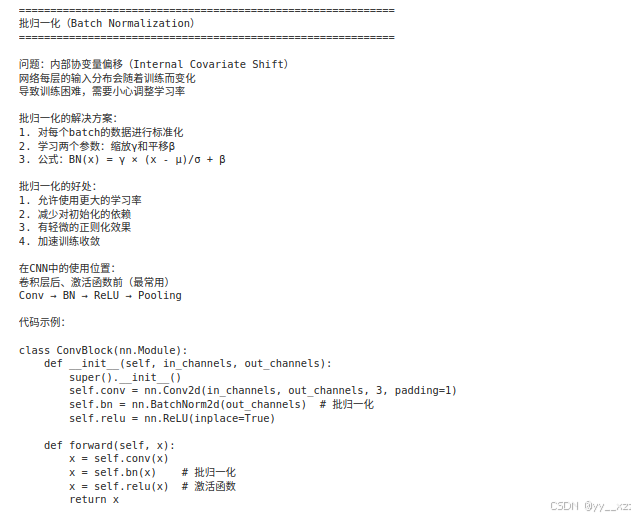

---

常见问题与解决方案

Q1: 如何设计CNN架构？

经验法则：

1. 从简单开始：先试3-5层的小网络
2. 使用小卷积核：3×3是最常用的尺寸
3. 逐步增加深度：每次增加1-2层，观察性能变化
4. 使用标准模块：如ResNet的残差块
5. 考虑感受野：确保最终感受野覆盖整个目标

Q2: 如何防止CNN过拟合？

策略：

1. 数据增强：旋转、翻转、裁剪、颜色变换
2. Dropout：在全连接层使用Dropout
3. 批归一化：有轻微的正则化效果
4. 权重衰减：L2正则化
5. 早停：监控验证集损失
6. 简化模型：减少参数数量

Q3: CNN学习率怎么设置？

建议：

1. 初始学习率：0.01（SGD）或0.001（Adam）
2. 学习率衰减：每30个epoch乘以0.1
3. 热身（Warmup）：前几个epoch线性增加学习率
4. 余弦退火：使用cosine学习率调度
5. 监控损失：如果损失不下降，适当降低学习率

Q4: 如何解释CNN的决策？

方法：

1. 特征可视化：可视化卷积核和特征图
2. CAM/Grad-CAM：生成类激活图
3. 遮挡测试：遮挡部分图像看预测变化
4. 敏感性分析：改变输入看输出变化

---

总结与练习

核心知识点总结：

1. 卷积操作：局部连接，权重共享
2. 池化操作：降维，增加平移不变性
3. 经典架构：LeNet, AlexNet, VGG, ResNet
4. 现代技巧：批归一化，Dropout，残差连接
5. 实践应用：图像分类，特征可视化

实操练习：

练习1：构建自定义CNN

# 尝试设计一个用于MNIST的CNN
class MyCNN(nn.Module):
    def __init__(self):
        super().__init__()
        # 你的设计
        pass
    
    def forward(self, x):
        # 前向传播
        pass

练习2：可视化训练过程

# 记录并可视化：
# 1. 每层的激活值分布
# 2. 梯度流
# 3. 权重分布

练习3：比较不同架构

# 比较以下架构在CIFAR-10上的性能：
# 1. 简单CNN（3层）
# 2. VGG风格（多个3×3卷积）
# 3. 带残差连接的CNN

练习4：实现数据增强

# 实现自定义数据增强：
# 1. 随机擦除（Random Erasing）
# 2. 混合图像（Mixup）
# 3. 颜色抖动（Color Jitter）

---