python
# This Python 3 environment comes with many helpful analytics libraries installed
# For example, here's several helpful packages to load

import numpy as np # linear algebra
import pandas as pd # data processing, CSV file I/O (e.g. pd.read_csv)

# Input data files are available in the read-only "../input/" directory
# For example, running this (by clicking run or pressing Shift+Enter) will list all files under the input directory

import os
for dirname, _, filenames in os.walk('/input'):
    for filename in filenames:
        print(os.path.join(dirname, filename))

# You can write up to 20GB to the current directory (/working/) that gets preserved as output when you create a version using "Save & Run All"
# You can also write temporary files to /temp/, but they won't be saved outside of the current session
python
/Amazon.csv
python
# Import necessary libraries
import numpy as np
import pandas as pd
import matplotlib.pyplot as plt
import seaborn as sns
import plotly.express as px
import plotly.graph_objects as go
from plotly.subplots import make_subplots
import warnings
warnings.filterwarnings('ignore')

# Set display options
pd.set_option('display.max_columns', None)
pd.set_option('display.max_rows', 100)
pd.set_option('display.float_format', '{:.2f}'.format)

# Set style for plots
plt.style.use('seaborn-v0_8-darkgrid')
sns.set_palette("husl")

# Load the dataset
df = pd.read_csv('/kaggle/input/amazon-sales-dataset/Amazon.csv')
1. 初始数据探索
python
# Basic information
print("\n1. DATASET DIMENSIONS:")
print(f"   Shape: {df.shape}")
print(f"   Total Records: {df.shape[0]:,}")
print(f" Total Features: {df.shape[1]}")1. DATASET DIMENSIONS:
Shape: (100000, 20)
Total Records: 100,000
Total Features: 20
python
# Display first few rows
print("\n2. FIRST 5 ROWS:")
display(df.head())

# Display last few rows
print("\n3. LAST 5 ROWS:")
display(df.tail())2. FIRST 5 ROWS:|---|------------|------------|------------|---------------|-----------|---------------------|-----------------|------------|----------|-----------|----------|-------|--------------|-------------|------------------|-------------|-------------|-------|---------------|-----------|
| | OrderID | OrderDate | CustomerID | CustomerName | ProductID | ProductName | Category | Brand | Quantity | UnitPrice | Discount | Tax | ShippingCost | TotalAmount | PaymentMethod | OrderStatus | City | State | Country | SellerID |
| 0 | ORD0000001 | 2023-01-31 | CUST001504 | Vihaan Sharma | P00014 | Drone Mini | Books | BrightLux | 3 | 106.59 | 0.00 | 0.00 | 0.09 | 319.86 | Debit Card | Delivered | Washington | DC | India | SELL01967 |
| 1 | ORD0000002 | 2023-12-30 | CUST000178 | Pooja Kumar | P00040 | Microphone | Home & Kitchen | UrbanStyle | 1 | 251.37 | 0.05 | 19.10 | 1.74 | 259.64 | Amazon Pay | Delivered | Fort Worth | TX | United States | SELL01298 |
| 2 | ORD0000003 | 2022-05-10 | CUST047516 | Sneha Singh | P00044 | Power Bank 20000mAh | Clothing | UrbanStyle | 3 | 35.03 | 0.10 | 7.57 | 5.91 | 108.06 | Debit Card | Delivered | Austin | TX | United States | SELL00908 |
| 3 | ORD0000004 | 2023-07-18 | CUST030059 | Vihaan Reddy | P00041 | Webcam Full HD | Home & Kitchen | Zenith | 5 | 33.58 | 0.15 | 11.42 | 5.53 | 159.66 | Cash on Delivery | Delivered | Charlotte | NC | India | SELL01164 |
| 4 | ORD0000005 | 2023-02-04 | CUST048677 | Aditya Kapoor | P00029 | T-Shirt | Clothing | KiddoFun | 2 | 515.64 | 0.25 | 38.67 | 9.23 | 821.36 | Credit Card | Cancelled | San Antonio | TX | Canada | SELL01411 |
3. LAST 5 ROWS:|-------|------------|------------|------------|---------------|-----------|-------------------|--------------------|-----------|----------|-----------|----------|--------|--------------|-------------|------------------|-------------|--------------|-------|---------------|-----------|
| | OrderID | OrderDate | CustomerID | CustomerName | ProductID | ProductName | Category | Brand | Quantity | UnitPrice | Discount | Tax | ShippingCost | TotalAmount | PaymentMethod | OrderStatus | City | State | Country | SellerID |
| 99995 | ORD0099996 | 2023-03-07 | CUST001356 | Karan Joshi | P00047 | Memory Card 128GB | Electronics | Apex | 2 | 492.34 | 0.00 | 78.77 | 2.75 | 1066.20 | UPI | Delivered | Jacksonville | FL | India | SELL00041 |
| 99996 | ORD0099997 | 2021-11-24 | CUST031254 | Sunita Kapoor | P00046 | Car Charger | Sports & Outdoors | Apex | 5 | 449.30 | 0.00 | 179.72 | 6.07 | 2432.29 | Credit Card | Delivered | San Jose | CA | United States | SELL01449 |
| 99997 | ORD0099998 | 2023-04-29 | CUST012579 | Aman Gupta | P00030 | Dress Shirt | Sports & Outdoors | BrightLux | 4 | 232.40 | 0.00 | 74.37 | 12.43 | 1016.40 | Cash on Delivery | Delivered | Indianapolis | IN | United States | SELL00028 |
| 99998 | ORD0099999 | 2021-11-01 | CUST026243 | Simran Gupta | P00046 | Car Charger | Sports & Outdoors | HomeEase | 1 | 294.05 | 0.00 | 23.52 | 13.09 | 330.66 | Debit Card | Delivered | Charlotte | NC | United States | SELL00324 |
| 99999 | ORD0100000 | 2021-12-04 | CUST029492 | Sunita Reddy | P00019 | LED Desk Lamp | Home & Kitchen | CoreTech | 5 | 166.70 | 0.05 | 63.35 | 3.34 | 858.52 | Debit Card | Delivered | New York | NY | United States | SELL00761 |
python
# Dataset information
print("\n4. DATASET INFORMATION:")
df.info()4. DATASET INFORMATION:
<class 'pandas.core.frame.DataFrame'>
RangeIndex: 100000 entries, 0 to 99999
Data columns (total 20 columns):
# Column Non-Null Count Dtype
--- ------ -------------- -----
0 OrderID 100000 non-null object
1 OrderDate 100000 non-null object
2 CustomerID 100000 non-null object
3 CustomerName 100000 non-null object
4 ProductID 100000 non-null object
5 ProductName 100000 non-null object
6 Category 100000 non-null object
7 Brand 100000 non-null object
8 Quantity 100000 non-null int64
9 UnitPrice 100000 non-null float64
10 Discount 100000 non-null float64
11 Tax 100000 non-null float64
12 ShippingCost 100000 non-null float64
13 TotalAmount 100000 non-null float64
14 PaymentMethod 100000 non-null object
15 OrderStatus 100000 non-null object
16 City 100000 non-null object
17 State 100000 non-null object
18 Country 100000 non-null object
19 SellerID 100000 non-null object
dtypes: float64(5), int64(1), object(14)
memory usage: 15.3+ MB
python
# Summary statistics for numerical columns
print("\n5. SUMMARY STATISTICS (Numerical Columns):")
display(df.describe())5. SUMMARY STATISTICS (Numerical Columns):|-------|-----------|-----------|-----------|-----------|--------------|-------------|
| | Quantity | UnitPrice | Discount | Tax | ShippingCost | TotalAmount |
| count | 100000.00 | 100000.00 | 100000.00 | 100000.00 | 100000.00 | 100000.00 |
| mean | 3.00 | 302.91 | 0.07 | 68.47 | 7.41 | 918.26 |
| std | 1.41 | 171.84 | 0.08 | 74.13 | 4.32 | 724.51 |
| min | 1.00 | 5.00 | 0.00 | 0.00 | 0.00 | 4.27 |
| 25% | 2.00 | 154.19 | 0.00 | 15.92 | 3.68 | 340.89 |
| 50% | 3.00 | 303.07 | 0.05 | 45.25 | 7.30 | 714.32 |
| 75% | 4.00 | 451.50 | 0.10 | 96.06 | 11.15 | 1349.76 |
| max | 5.00 | 599.99 | 0.30 | 538.46 | 15.00 | 3534.98 |
python
# Summary statistics for categorical columns
print("\n6. SUMMARY STATISTICS (Categorical Columns):")
categorical_cols = df.select_dtypes(include=['object']).columns
for col in categorical_cols:
    print(f"\n{col}:")
    print(f"   Unique values: {df[col].nunique()}")
    print(f"   Top 5 values:")
display(df[col].value_counts().head())6. SUMMARY STATISTICS (Categorical Columns):
OrderID:
Unique values: 100000
Top 5 values:
OrderID
ORD0000001 1
ORD0066651 1
ORD0066673 1
ORD0066672 1
ORD0066671 1
Name: count, dtype: int64
OrderDate:
Unique values: 1825
Top 5 values:
OrderDate
2022-04-28 85
2021-01-21 82
2021-09-09 79
2022-01-31 79
2024-03-22 78
Name: count, dtype: int64
CustomerID:
Unique values: 43233
Top 5 values:
CustomerID
CUST023748 10
CUST037103 10
CUST042938 9
CUST009614 9
CUST034288 9
Name: count, dtype: int64
CustomerName:
Unique values: 200
Top 5 values:
CustomerName
Karan Joshi 556
Arjun Kumar 553
Pooja Kapoor 552
Rohit Gupta 547
Vihaan Singh 544
Name: count, dtype: int64
ProductID:
Unique values: 50
Top 5 values:
ProductID
P00019 2098
P00022 2088
P00023 2058
P00017 2054
P00037 2054
Name: count, dtype: int64
ProductName:
Unique values: 50
Top 5 values:
ProductName
LED Desk Lamp 2098
Water Bottle 2088
Cookware Set 2058
Electric Kettle 2054
Router 2054
Name: count, dtype: int64
Category:
Unique values: 6
Top 5 values:
Category
Electronics 16853
Sports & Outdoors 16804
Books 16752
Home & Kitchen 16610
Toys & Games 16542
Name: count, dtype: int64
Brand:
Unique values: 10
Top 5 values:
Brand
ReadMore 10204
FitLife 10147
CoreTech 10127
KiddoFun 10077
Zenith 9990
Name: count, dtype: int64
PaymentMethod:
Unique values: 6
Top 5 values:
PaymentMethod
Credit Card 35038
Debit Card 20024
UPI 15066
Amazon Pay 15017
Net Banking 9927
Name: count, dtype: int64
OrderStatus:
Unique values: 5
Top 5 values:
OrderStatus
Delivered 74628
Shipped 15192
Pending 4103
Returned 3049
Cancelled 3028
Name: count, dtype: int64
City:
Unique values: 20
Top 5 values:
City
Charlotte 5110
San Jose 5107
Jacksonville 5107
Dallas 5105
Los Angeles 5058
Name: count, dtype: int64
State:
Unique values: 13
Top 5 values:
State
TX 24896
CA 19921
NC 5110
FL 5107
WA 5039
Name: count, dtype: int64
Country:
Unique values: 5
Top 5 values:
Country
United States 70058
India 15051
Canada 5818
United Kingdom 4943
Australia 4130
Name: count, dtype: int64
SellerID:
Unique values: 1999
Top 5 values:
SellerID
SELL01099 78
SELL01335 71
SELL00792 71
SELL00536 70
SELL01447 70
Name: count, dtype: int642. 数据清理与整理
python
# Check for missing values
print("\n1. MISSING VALUES CHECK:")
missing_data = df.isnull().sum()
missing_percentage = (missing_data / len(df)) * 100
missing_df = pd.DataFrame({
    'Missing Values': missing_data,
    'Percentage': missing_percentage
})
missing_df = missing_df[missing_df['Missing Values'] > 0]
if len(missing_df) > 0:
    display(missing_df)
else:
print(" No missing values found! ✓")1. MISSING VALUES CHECK:
No missing values found! ✓
python
# Check for duplicates
print("\n2. DUPLICATE RECORDS CHECK:")
duplicates = df.duplicated().sum()
print(f"   Duplicate rows: {duplicates}")
if duplicates > 0:
    df = df.drop_duplicates()
print(f" Removed {duplicates} duplicate rows")2. DUPLICATE RECORDS CHECK:
Duplicate rows: 0
python
# Check data types and convert
print("\n3. DATA TYPE VALIDATION:")
# Convert OrderDate to datetime
df['OrderDate'] = pd.to_datetime(df['OrderDate'])
print(" Converted OrderDate to datetime format ✓")3. DATA TYPE VALIDATION:
Converted OrderDate to datetime format ✓
python
# Extract date components for analysis
df['OrderYear'] = df['OrderDate'].dt.year
df['OrderMonth'] = df['OrderDate'].dt.month
df['OrderMonthName'] = df['OrderDate'].dt.strftime('%B')
df['OrderQuarter'] = df['OrderDate'].dt.quarter
df['OrderWeekday'] = df['OrderDate'].dt.day_name()
df['OrderDay'] = df['OrderDate'].dt.day
python
# Check for inconsistent data
print("\n4. DATA CONSISTENCY CHECK:")
# Check for negative values in numerical columns
numerical_cols = ['Quantity', 'UnitPrice', 'Discount', 'Tax', 'ShippingCost', 'TotalAmount']
for col in numerical_cols:
    negative_count = (df[col] < 0).sum()
    if negative_count > 0:
print(f" Warning: {negative_count} negative values found in {col}")4. DATA CONSISTENCY CHECK:
python
# Check for zero or extremely low prices
zero_price = (df['UnitPrice'] <= 0).sum()
print(f" Products with zero/negative price: {zero_price}") Products with zero/negative price: 0
python
# Calculate derived metrics
df['DiscountAmount'] = df['UnitPrice'] * df['Quantity'] * df['Discount']
df['NetAmount'] = df['TotalAmount'] - df['Tax'] - df['ShippingCost']
df['ProfitMargin'] = ((df['TotalAmount'] - (df['UnitPrice'] * df['Quantity'])) / (df['UnitPrice'] * df['Quantity'])) * 100
python
# Create order status categories
df['OrderStatusCategory'] = df['OrderStatus'].apply(
    lambda x: 'Completed' if x == 'Delivered' else
             'In Progress' if x in ['Shipped', 'Pending'] else
             'Failed' if x in ['Cancelled', 'Returned'] else 'Other'
)
python
# Create customer segments based on total spending
customer_totals = df.groupby('CustomerID')['TotalAmount'].sum().reset_index()
customer_totals['CustomerSegment'] = pd.qcut(customer_totals['TotalAmount'],
                                             q=4,
                                             labels=['Low Spender', 'Medium Spender', 'High Spender', 'VIP'])
df = df.merge(customer_totals[['CustomerID', 'CustomerSegment']], on='CustomerID', how='left')

print("\n5. DATA WRANGLING COMPLETED!")
print("   Added features: OrderYear, OrderMonth, OrderMonthName, OrderQuarter,")
print("   OrderWeekday, OrderDay, DiscountAmount, NetAmount, ProfitMargin,")
print(" OrderStatusCategory, CustomerSegment")5. DATA WRANGLING COMPLETED!
Added features: OrderYear, OrderMonth, OrderMonthName, OrderQuarter,
OrderWeekday, OrderDay, DiscountAmount, NetAmount, ProfitMargin,
OrderStatusCategory, CustomerSegment3. 探索性数据分析 - 图形展示
python
# Set up the figure for subplots
fig = plt.figure(figsize=(20, 16))

print("\n1. SALES TREND OVER TIME")
ax1 = plt.subplot(3, 3, 1)
monthly_sales = df.groupby(['OrderYear', 'OrderMonth'])['TotalAmount'].sum().reset_index()

monthly_sales['Date'] = pd.to_datetime(
    monthly_sales['OrderYear'].astype(str) + '-' +
    monthly_sales['OrderMonth'].astype(str) + '-01'
)
monthly_sales.set_index('Date')['TotalAmount'].plot(ax=ax1, color='#2E86AB', linewidth=2)
ax1.set_title('Monthly Sales Trend', fontsize=14, fontweight='bold', pad=20)
ax1.set_xlabel('Date')
ax1.set_ylabel('Total Sales Amount')
ax1.grid(True, alpha=0.3)
ax1.tick_params(axis='x', rotation=45)

plt.show()1. SALES TREND OVER TIME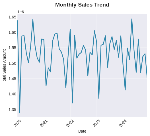
python
# 2. Sales by Year
fig, ax2 = plt.subplots(figsize=(10, 5))
yearly_sales = df.groupby('OrderYear')['TotalAmount'].sum()
yearly_sales.plot(kind='bar', ax=ax2, color='#A23B72', edgecolor='black')
ax2.set_title('Yearly Sales Comparison', fontsize=14, fontweight='bold', pad=20)
ax2.set_xlabel('Year')
ax2.set_ylabel('Total Sales Amount')
ax2.tick_params(axis='x', rotation=45)
for i, v in enumerate(yearly_sales.values):
    ax2.text(i, v, f'{v:,.0f}', ha='center', va='bottom', fontsize=9)

plt.tight_layout()
plt.show()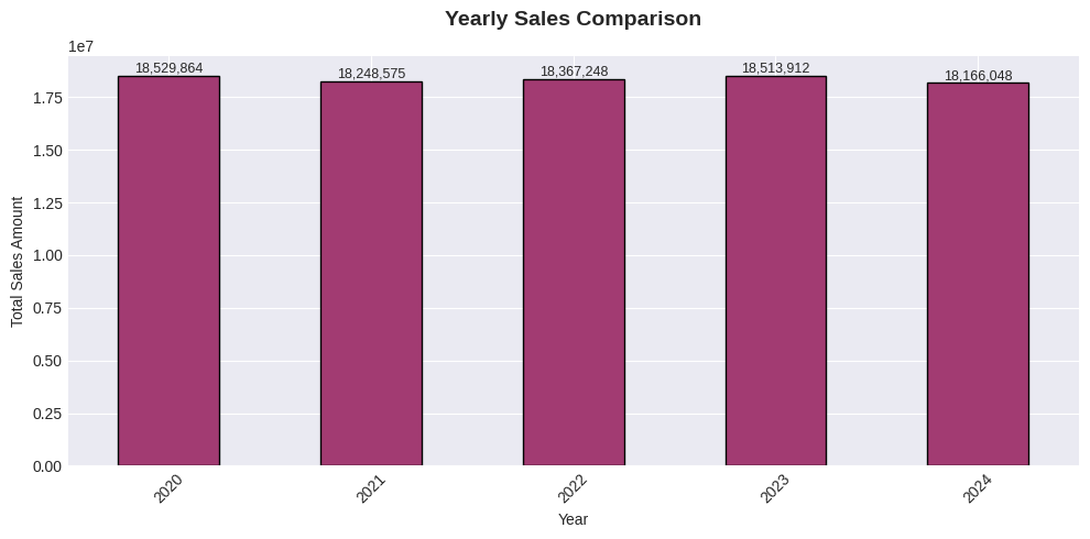
python
# 3. Top 10 Products by Sales
fig, ax3 = plt.subplots(figsize=(10, 5))
top_products = df.groupby('ProductName')['TotalAmount'].sum().nlargest(10).sort_values()
top_products.plot(kind='barh', ax=ax3, color='#F18F01')
ax3.set_title('Top 10 Products by Sales', fontsize=14, fontweight='bold', pad=20)
ax3.set_xlabel('Total Sales Amount')


plt.show()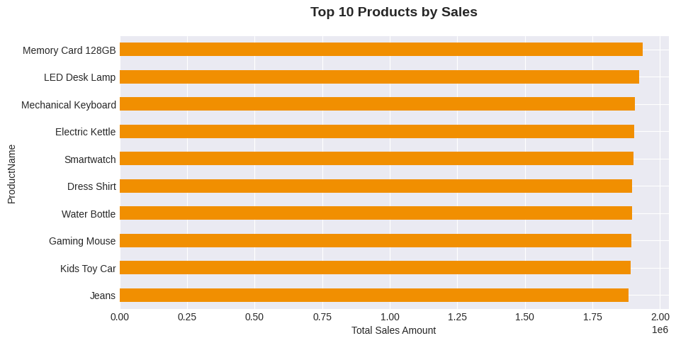
python
# 4. Sales by Category
fig, ax4 = plt.subplots(figsize=(10, 5))
category_sales = df.groupby('Category')['TotalAmount'].sum().sort_values(ascending=False)
category_sales.plot(kind='bar', ax=ax4, color='#73AB84', edgecolor='black')
ax4.set_title('Sales by Product Category', fontsize=14, fontweight='bold', pad=20)
ax4.set_xlabel('Category')
ax4.set_ylabel('Total Sales Amount')
ax4.tick_params(axis='x', rotation=45)

plt.tight_layout()
plt.show()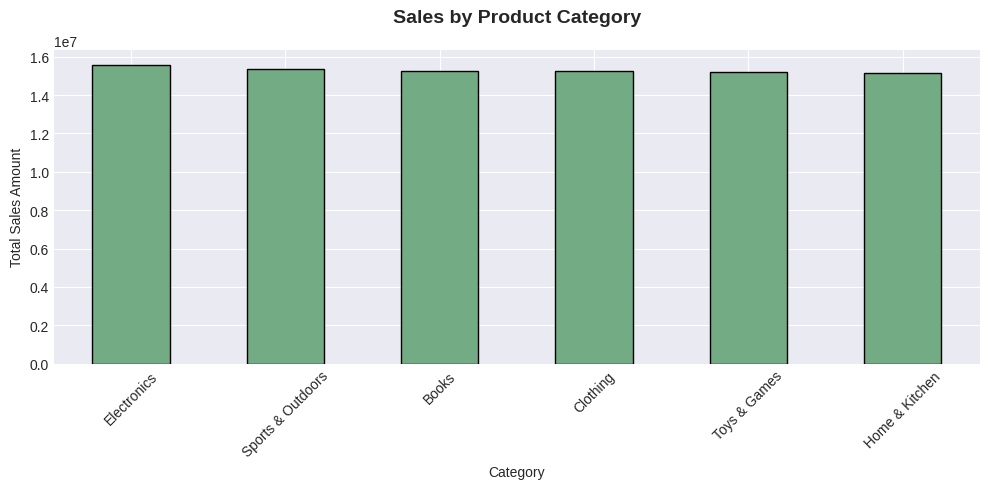
python
# 5. Order Status Distribution
fig, ax5 = plt.subplots(figsize=(10, 5))
status_counts = df['OrderStatus'].value_counts()
colors = ['#2E86AB', '#A23B72', '#F18F01', '#73AB84', '#C73E1D']
wedges, texts, autotexts = ax5.pie(status_counts.values, labels=status_counts.index,
                                   autopct='%1.1f%%', startangle=90, colors=colors,
                                   wedgeprops={'edgecolor': 'black', 'linewidth': 1})
ax5.set_title('Order Status Distribution', fontsize=14, fontweight='bold', pad=20)
plt.setp(autotexts, size=10, weight="bold", color='white')

plt.tight_layout()
plt.show()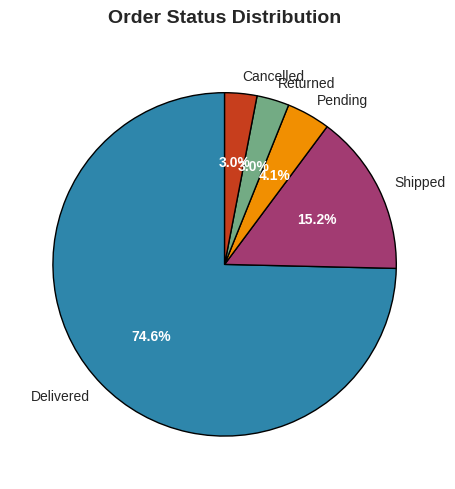
python
# 6. Payment Method Distribution
fig, ax6 = plt.subplots(figsize=(10, 5))
payment_counts = df['PaymentMethod'].value_counts()
payment_counts.plot(kind='bar', ax=ax6, color='#5B8C5A', edgecolor='black')
ax6.set_title('Payment Method Distribution', fontsize=14, fontweight='bold', pad=20)
ax6.set_xlabel('Payment Method')
ax6.set_ylabel('Number of Orders')
ax6.tick_params(axis='x', rotation=45)
for i, v in enumerate(payment_counts.values):
    ax6.text(i, v, str(v), ha='center', va='bottom', fontsize=9)

plt.tight_layout()
plt.show()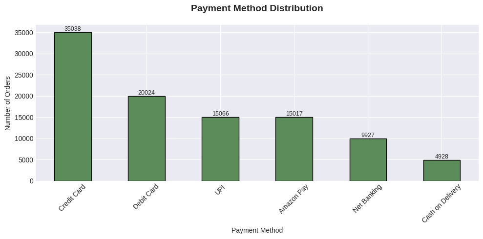
python
# 7. Top 10 Customers by Total Spending
fig, ax7 = plt.subplots(figsize=(10, 5))
top_customers = df.groupby('CustomerName')['TotalAmount'].sum().nlargest(10).sort_values()
top_customers.plot(kind='barh', ax=ax7, color='#C73E1D')
ax7.set_title('Top 10 Customers by Spending', fontsize=14, fontweight='bold', pad=20)
ax7.set_xlabel('Total Amount Spent')

plt.tight_layout()
plt.show()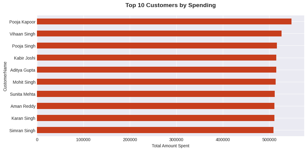
python
# 8. Sales by Country
fig, ax8 = plt.subplots(figsize=(10, 5))
country_sales = df.groupby('Country')['TotalAmount'].sum().sort_values(ascending=False)
country_sales.plot(kind='bar', ax=ax8, color='#2E86AB', edgecolor='black')
ax8.set_title('Sales by Country', fontsize=14, fontweight='bold', pad=20)
ax8.set_xlabel('Country')
ax8.set_ylabel('Total Sales Amount')
ax8.tick_params(axis='x', rotation=45)

plt.tight_layout()
plt.show()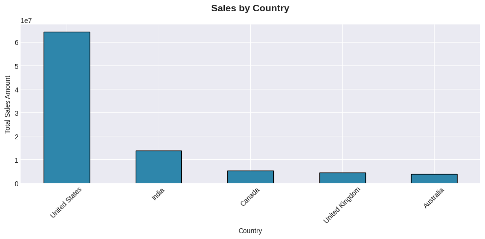
python
# 9. Brand Performance
fig, ax9 = plt.subplots(figsize=(10, 5))
top_brands = df.groupby('Brand')['TotalAmount'].sum().nlargest(10).sort_values()
top_brands.plot(kind='barh', ax=ax9, color='#A23B72')
ax9.set_title('Top 10 Brands by Sales', fontsize=14, fontweight='bold', pad=20)
ax9.set_xlabel('Total Sales Amount')

plt.tight_layout()
plt.show()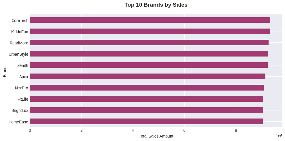
4. 使用 Plotly 进行高级可视化展示
python
# 1. Interactive Sales Trend with Plotly
print("\n1. INTERACTIVE SALES TREND")
fig1 = make_subplots(rows=2, cols=2,
                     subplot_titles=('Monthly Sales Trend', 'Sales by Quarter',
                                     'Daily Sales Pattern', 'Year-over-Year Growth'),
                     vertical_spacing=0.12,
                     horizontal_spacing=0.1)

# CORRECTED: Monthly sales trend - FIXED THIS LINE
monthly_data = df.groupby(['OrderYear', 'OrderMonth'])['TotalAmount'].sum().reset_index()
# Fix the datetime creation - THIS IS THE CRITICAL FIX
monthly_data['Date'] = pd.to_datetime(
    monthly_data['OrderYear'].astype(str) + '-' +
    monthly_data['OrderMonth'].astype(str) + '-01'
)

fig1.add_trace(go.Scatter(x=monthly_data['Date'], y=monthly_data['TotalAmount'],
                         mode='lines+markers', name='Monthly Sales',
                         line=dict(color='#2E86AB', width=3)),
               row=1, col=1)

# Sales by quarter
quarterly_sales = df.groupby(['OrderYear', 'OrderQuarter'])['TotalAmount'].sum().reset_index()
for year in quarterly_sales['OrderYear'].unique():
    year_data = quarterly_sales[quarterly_sales['OrderYear'] == year]
    fig1.add_trace(go.Bar(x=year_data['OrderQuarter'], y=year_data['TotalAmount'],
                         name=f'{year}', opacity=0.7),
                   row=1, col=2)

# Daily sales pattern
daily_sales = df.groupby('OrderDay')['TotalAmount'].sum()
fig1.add_trace(go.Bar(x=daily_sales.index, y=daily_sales.values,
                     marker_color='#F18F01'),
               row=2, col=1)

# Year-over-year growth
yearly_growth = df.groupby('OrderYear')['TotalAmount'].sum().pct_change() * 100
fig1.add_trace(go.Scatter(x=yearly_growth.index, y=yearly_growth.values,
                         mode='lines+markers+text',
                         text=[f'{val:.1f}%' for val in yearly_growth.values],
                         textposition='top center',
                         line=dict(color='#73AB84', width=3, dash='dot')),
               row=2, col=2)

fig1.update_layout(height=800, title_text="Sales Performance Analysis",
                  showlegend=True, template='plotly_white')
fig1.show()1. INTERACTIVE SALES TREND
python
# 2. Geographic Sales Analysis
print("\n2. GEOGRAPHIC SALES ANALYSIS")
geo_data = df.groupby(['Country', 'State'])['TotalAmount'].sum().reset_index()
fig2 = px.treemap(geo_data, path=['Country', 'State'], values='TotalAmount',
                  color='TotalAmount', hover_data=['TotalAmount'],
                  color_continuous_scale='Viridis',
                  title='Sales Distribution by Country and State')
fig2.update_layout(margin=dict(t=50, l=25, r=25, b=25))
fig2.show()2. GEOGRAPHIC SALES ANALYSIS
python
# 3. Customer Segmentation Analysis
print("\n3. CUSTOMER SEGMENTATION ANALYSIS")
segment_data = df.groupby(['CustomerSegment', 'OrderStatusCategory'])['TotalAmount'].sum().reset_index()
fig3 = px.sunburst(segment_data, path=['CustomerSegment', 'OrderStatusCategory'],
                   values='TotalAmount',
                   color='TotalAmount', hover_data=['TotalAmount'],
                   color_continuous_scale='RdBu',
                   title='Customer Segmentation by Spending and Order Status')
fig3.update_layout(margin=dict(t=50, l=25, r=25, b=25))
fig3.show()3. CUSTOMER SEGMENTATION ANALYSIS
python
# 4. Correlation Heatmap
print("\n4. FEATURE CORRELATION HEATMAP")
# Select numerical features for correlation
numerical_features = ['Quantity', 'UnitPrice', 'Discount', 'Tax',
                      'ShippingCost', 'TotalAmount', 'NetAmount', 'ProfitMargin']
correlation_matrix = df[numerical_features].corr()

fig4 = go.Figure(data=go.Heatmap(
    z=correlation_matrix.values,
    x=correlation_matrix.columns,
    y=correlation_matrix.columns,
    colorscale='RdBu',
    zmin=-1, zmax=1,
    text=correlation_matrix.round(2).values,
    texttemplate='%{text}',
    textfont={"size": 10},
    hoverongaps=False))

fig4.update_layout(
    title='Feature Correlation Heatmap',
    xaxis_title="Features",
    yaxis_title="Features",
    height=600,
    width=800,
    template='plotly_white'
)
fig4.show()4. FEATURE CORRELATION HEATMAP5. 高级分析与洞察力
python
print("\n" + "="*80)
print("ADVANCED ANALYTICS AND INSIGHTS")
print("="*80)

# 1. Customer Lifetime Value Analysis
print("\n1. CUSTOMER LIFETIME VALUE ANALYSIS")
customer_analysis = df.groupby('CustomerID').agg({
    'OrderID': 'count',
    'TotalAmount': ['sum', 'mean'],
    'OrderDate': ['min', 'max']
}).round(2)

customer_analysis.columns = ['TotalOrders', 'TotalSpent', 'AvgOrderValue',
                            'FirstPurchase', 'LastPurchase']
customer_analysis['DaysActive'] = (pd.to_datetime(customer_analysis['LastPurchase']) -
                                   pd.to_datetime(customer_analysis['FirstPurchase'])).dt.days
customer_analysis['CLV'] = customer_analysis['TotalSpent'] / customer_analysis['TotalOrders']

print("Top 10 Customers by CLV:")
display(customer_analysis.nlargest(10, 'CLV')[['TotalOrders', 'TotalSpent', 'CLV', 'DaysActive']])

# 2. Product Performance Analysis
print("\n2. PRODUCT PERFORMANCE ANALYSIS")
product_performance = df.groupby(['ProductName', 'Category', 'Brand']).agg({
    'OrderID': 'count',
    'Quantity': 'sum',
    'TotalAmount': 'sum',
    'UnitPrice': 'mean'
}).round(2)

product_performance.columns = ['OrdersCount', 'TotalQuantity', 'TotalRevenue', 'AvgPrice']
product_performance['RevenuePerOrder'] = (product_performance['TotalRevenue'] /
                                         product_performance['OrdersCount'])

print("Top 10 Products by Revenue:")
display(product_performance.nlargest(10, 'TotalRevenue'))

# 3. Seasonality Analysis
print("\n3. SEASONALITY ANALYSIS")
monthly_analysis = df.groupby(['OrderYear', 'OrderMonth', 'OrderMonthName']).agg({
    'OrderID': 'count',
    'TotalAmount': 'sum',
    'Quantity': 'sum'
}).reset_index()

monthly_analysis['AvgOrderValue'] = monthly_analysis['TotalAmount'] / monthly_analysis['OrderID']
monthly_analysis['Date'] = pd.to_datetime(
    monthly_analysis['OrderYear'].astype(str) + '-' +
    monthly_analysis['OrderMonth'].astype(str) + '-01'
)

print("Best Performing Months:")
best_months = monthly_analysis.nlargest(5, 'TotalAmount')
display(best_months[['OrderYear', 'OrderMonthName', 'OrderID', 'TotalAmount', 'AvgOrderValue']])

# 4. Payment Method Analysis
print("\n4. PAYMENT METHOD ANALYSIS")
payment_analysis = df.groupby('PaymentMethod').agg({
    'OrderID': 'count',
    'TotalAmount': ['sum', 'mean', 'std'],
    'Discount': 'mean'
}).round(2)

payment_analysis.columns = ['OrdersCount', 'TotalRevenue', 'AvgOrderValue',
                           'StdOrderValue', 'AvgDiscount']
payment_analysis['RevenueShare'] = (payment_analysis['TotalRevenue'] /
                                   payment_analysis['TotalRevenue'].sum() * 100).round(2)

print("Payment Method Performance:")
display(payment_analysis)

# 5. Return/Cancellation Analysis
print("\n5. RETURN/CANCELLATION ANALYSIS")
failed_orders = df[df['OrderStatus'].isin(['Cancelled', 'Returned'])]
if len(failed_orders) > 0:
    failure_analysis = failed_orders.groupby(['OrderStatus', 'Category']).agg({
        'OrderID': 'count',
        'TotalAmount': 'sum'
    }).reset_index()

    failure_analysis['FailureRate'] = (failure_analysis['OrderID'] /
                                      failure_analysis['OrderID'].sum() * 100).round(2)

    print("Failure Analysis by Category:")
    display(failure_analysis.sort_values('FailureRate', ascending=False))
else:
print("No cancelled or returned orders found.")================================================================================
ADVANCED ANALYTICS AND INSIGHTS
================================================================================
1. CUSTOMER LIFETIME VALUE ANALYSIS
Top 10 Customers by CLV:|------------|-------------|------------|---------|------------|
| | TotalOrders | TotalSpent | CLV | DaysActive |
| CustomerID | | | | |
| CUST010791 | 1 | 3484.44 | 3484.44 | 0 |
| CUST030934 | 1 | 3439.11 | 3439.11 | 0 |
| CUST021621 | 1 | 3385.69 | 3385.69 | 0 |
| CUST012476 | 1 | 3366.38 | 3366.38 | 0 |
| CUST014210 | 1 | 3344.38 | 3344.38 | 0 |
| CUST010357 | 1 | 3342.39 | 3342.39 | 0 |
| CUST012933 | 1 | 3290.92 | 3290.92 | 0 |
| CUST016507 | 1 | 3284.42 | 3284.42 | 0 |
| CUST035792 | 1 | 3283.13 | 3283.13 | 0 |
| CUST046858 | 1 | 3265.73 | 3265.73 | 0 |
2. PRODUCT PERFORMANCE ANALYSIS
Top 10 Products by Revenue:
|---------------------|--------------------|----------|-------------|---------------|--------------|----------|-----------------|
| | | | OrdersCount | TotalQuantity | TotalRevenue | AvgPrice | RevenuePerOrder |
| ProductName | Category | Brand | | | | | |
| Desk Organizer | Clothing | KiddoFun | 58 | 166 | 58059.53 | 348.71 | 1001.03 |
| Jeans | Sports & Outdoors | Apex | 50 | 156 | 56329.85 | 361.23 | 1126.60 |
| Memory Card 128GB | Home & Kitchen | HomeEase | 53 | 162 | 55874.05 | 341.49 | 1054.23 |
| Cookware Set | Books | KiddoFun | 43 | 147 | 53889.96 | 379.81 | 1253.25 |
| HDMI Cable 2m | Electronics | Zenith | 48 | 154 | 53200.52 | 334.98 | 1108.34 |
| LED Desk Lamp | Sports & Outdoors | Apex | 52 | 167 | 52494.29 | 317.06 | 1009.51 |
| 4K Monitor | Sports & Outdoors | ReadMore | 59 | 181 | 52452.39 | 279.35 | 889.02 |
| USB-C Charger | Sports & Outdoors | Zenith | 47 | 141 | 52155.04 | 358.60 | 1109.68 |
| Mechanical Keyboard | Home & Kitchen | HomeEase | 43 | 144 | 51373.57 | 371.08 | 1194.73 |
| LED Desk Lamp | Toys & Games | CoreTech | 43 | 155 | 51046.67 | 308.91 | 1187.13 |
3. SEASONALITY ANALYSIS
Best Performing Months:
|----|-----------|----------------|---------|-------------|---------------|
| | OrderYear | OrderMonthName | OrderID | TotalAmount | AvgOrderValue |
| 52 | 2024 | May | 1753 | 1642609.94 | 937.03 |
| 7 | 2020 | August | 1783 | 1640874.93 | 920.29 |
| 0 | 2020 | January | 1730 | 1637069.40 | 946.28 |
| 24 | 2022 | January | 1744 | 1609759.87 | 923.03 |
| 35 | 2022 | December | 1753 | 1604276.23 | 915.16 |
4. PAYMENT METHOD ANALYSIS
Payment Method Performance:
|------------------|-------------|--------------|---------------|---------------|-------------|--------------|
| | OrdersCount | TotalRevenue | AvgOrderValue | StdOrderValue | AvgDiscount | RevenueShare |
| PaymentMethod | | | | | | |
| Amazon Pay | 15017 | 13697498.42 | 912.13 | 724.07 | 0.07 | 14.92 |
| Cash on Delivery | 4928 | 4515609.16 | 916.32 | 714.06 | 0.07 | 4.92 |
| Credit Card | 35038 | 32122158.69 | 916.78 | 725.14 | 0.07 | 34.98 |
| Debit Card | 20024 | 18538678.53 | 925.82 | 728.42 | 0.07 | 20.19 |
| Net Banking | 9927 | 9055674.57 | 912.23 | 722.90 | 0.07 | 9.86 |
| UPI | 15066 | 13896028.55 | 922.34 | 722.70 | 0.07 | 15.13 |
5. RETURN/CANCELLATION ANALYSIS
Failure Analysis by Category:
|----|-------------|--------------------|---------|-------------|-------------|
| | OrderStatus | Category | OrderID | TotalAmount | FailureRate |
| 2 | Cancelled | Electronics | 544 | 500092.66 | 8.95 |
| 9 | Returned | Home & Kitchen | 534 | 504832.21 | 8.79 |
| 6 | Returned | Books | 523 | 468272.20 | 8.61 |
| 10 | Returned | Sports & Outdoors | 518 | 438585.17 | 8.52 |
| 5 | Cancelled | Toys & Games | 512 | 499510.16 | 8.43 |
| 3 | Cancelled | Home & Kitchen | 508 | 479301.17 | 8.36 |
| 7 | Returned | Clothing | 504 | 484607.10 | 8.29 |
| 0 | Cancelled | Books | 500 | 463255.99 | 8.23 |
| 4 | Cancelled | Sports & Outdoors | 497 | 472861.93 | 8.18 |
| 11 | Returned | Toys & Games | 495 | 463854.64 | 8.15 |
| 8 | Returned | Electronics | 475 | 420511.14 | 7.82 |
| 1 | Cancelled | Clothing | 467 | 436100.48 | 7.68 |
6. 关键指标与总结
python
print("\n" + "="*80)
print("KEY BUSINESS METRICS SUMMARY")
print("="*80)

# Calculate key metrics
total_revenue = df['TotalAmount'].sum()
total_orders = df['OrderID'].nunique()
total_customers = df['CustomerID'].nunique()
total_products = df['ProductID'].nunique()
avg_order_value = total_revenue / total_orders
success_rate = (df[df['OrderStatus'] == 'Delivered'].shape[0] / total_orders) * 100

# Revenue by year
revenue_by_year = df.groupby('OrderYear')['TotalAmount'].sum()

# Top categories
top_categories = df.groupby('Category')['TotalAmount'].sum().nlargest(3)

# Top products
top_products = df.groupby('ProductName')['TotalAmount'].sum().nlargest(3)

# Top customers
top_customers = df.groupby('CustomerName')['TotalAmount'].sum().nlargest(3)

print(f"""
OVERALL PERFORMANCE:
{'-'*40}
• Total Revenue: ${total_revenue:,.2f}
• Total Orders: {total_orders:,}
• Total Customers: {total_customers:,}
• Total Products: {total_products:,}
• Average Order Value: ${avg_order_value:,.2f}
• Order Success Rate: {success_rate:.1f}%

TOP PERFORMERS:
{'-'*40}
Top 3 Categories:
  1. {top_categories.index[0]} (${top_categories.iloc[0]:,.2f})
  2. {top_categories.index[1]} (${top_categories.iloc[1]:,.2f})
  3. {top_categories.index[2]} (${top_categories.iloc[2]:,.2f})

Top 3 Products:
  1. {top_products.index[0]} (${top_products.iloc[0]:,.2f})
  2. {top_products.index[1]} (${top_products.iloc[1]:,.2f})
  3. {top_products.index[2]} (${top_products.iloc[2]:,.2f})

Top 3 Customers:
  1. {top_customers.index[0]} (${top_customers.iloc[0]:,.2f})
  2. {top_customers.index[1]} (${top_customers.iloc[1]:,.2f})
  3. {top_customers.index[2]} (${top_customers.iloc[2]:,.2f})

YEARLY REVENUE:
{'-'*40}
""")

for year, revenue in revenue_by_year.items():
    print(f"  {year}: ${revenue:,.2f}")

print(f"""
BUSINESS INSIGHTS:
{'-'*40}
1. Best Performing Year: {revenue_by_year.idxmax()} (${revenue_by_year.max():,.2f})
2. Most Popular Category: {top_categories.index[0]}
3. Most Valuable Product: {top_products.index[0]}
4. Most Loyal Customer: {top_customers.index[0]}
5. Best Payment Method: {df['PaymentMethod'].value_counts().index[0]}
6. Busiest Month: {df['OrderMonthName'].value_counts().index[0]}
""")================================================================================
KEY BUSINESS METRICS SUMMARY
================================================================================
OVERALL PERFORMANCE:
----------------------------------------
• Total Revenue: $91,825,647.92
• Total Orders: 100,000
• Total Customers: 43,233
• Total Products: 50
• Average Order Value: $918.26
• Order Success Rate: 74.6%
TOP PERFORMERS:
----------------------------------------
Top 3 Categories:
1. Electronics ($15,584,217.18)
2. Sports & Outdoors ($15,345,571.88)
3. Books ($15,261,837.01)
Top 3 Products:
1. Memory Card 128GB ($1,935,138.40)
2. LED Desk Lamp ($1,921,948.41)
3. Mechanical Keyboard ($1,906,963.54)
Top 3 Customers:
1. Pooja Kapoor ($547,832.64)
2. Vihaan Singh ($526,675.89)
3. Pooja Singh ($516,451.45)
YEARLY REVENUE:
----------------------------------------
2020: $18,529,864.02
2021: $18,248,574.81
2022: $18,367,248.41
2023: $18,513,912.19
2024: $18,166,048.49
BUSINESS INSIGHTS:
----------------------------------------
1. Best Performing Year: 2020 ($18,529,864.02)
2. Most Popular Category: Electronics
3. Most Valuable Product: Memory Card 128GB
4. Most Loyal Customer: Pooja Kapoor
5. Best Payment Method: Credit Card
6. Busiest Month: August