极限的常数倍数性质证明和可视化代码
flyfish
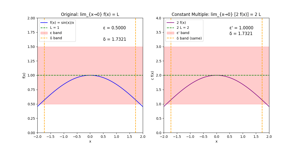
原函数f(x)=sin(x)xf(x) = \frac{\sin(x)}{x}f(x)=xsin(x),极限点a=0a = 0a=0,极限值L=1L = 1L=1,常数c=2c = 2c=2。
避免x=0x = 0x=0处的除零错误。
左侧:原函数f(x);右侧:c * f(x)。
左侧:x范围-2, 2,y范围0, 2;绘制f(x)曲线(蓝色)、极限线y=1(绿色虚线)。
右侧:y范围调整为0, 4(因c=2缩放);绘制c*f(x)曲线(紫色)、极限线y=2(绿色虚线)。
每个子图有ϵ\epsilonϵ带(红色半透明水平带,表示函数值在L ± ϵ\epsilonϵ或cL ± ϵ\epsilonϵ'内的范围)。
δ\deltaδ带(两条橙色虚线,表示x在a ± δ\deltaδ内的范围)。
证明极限的常数倍数性质:如果 limx→af(x)=L\lim_{x \to a} f(x) = Llimx→af(x)=L,且 ccc 是与 xxx 无关的常数,则 limx→ac⋅f(x)=c⋅L\lim_{x \to a} c \\cdot f(x) = c \cdot Lx→alimc⋅f(x)=c⋅L
证明前提
假设 limx→af(x)=L\lim_{x \to a} f(x) = Llimx→af(x)=L,这意味着:对于任意给定的正数 ϵ>0\epsilon > 0ϵ>0,总存在正数 δ>0\delta > 0δ>0,使得当 0<∣x−a∣<δ0 < |x - a| < \delta0<∣x−a∣<δ 时,有 ∣f(x)−L∣<ϵ|f(x) - L| < \epsilon∣f(x)−L∣<ϵ。
ccc 是常数(可以是正、负或零)。
证明目标
需要证明:对于函数 g(x)=c⋅f(x)g(x) = c \cdot f(x)g(x)=c⋅f(x),limx→ag(x)=c⋅L\lim_{x \to a} g(x) = c \cdot Llimx→ag(x)=c⋅L。即,对于任意给定的正数 ϵ′>0\epsilon' > 0ϵ′>0,总存在正数 δ′>0\delta' > 0δ′>0,使得当 0<∣x−a∣<δ′0 < |x - a| < \delta'0<∣x−a∣<δ′ 时,有 ∣g(x)−cL∣<ϵ′|g(x) - c L| < \epsilon'∣g(x)−cL∣<ϵ′。
步骤 1: 处理特殊情况 c=0c = 0c=0
如果 c=0c = 0c=0,则 g(x)=0⋅f(x)=0g(x) = 0 \cdot f(x) = 0g(x)=0⋅f(x)=0(恒为 0),所以 limx→ag(x)=0=0⋅L=c⋅L\lim_{x \to a} g(x) = 0 = 0 \cdot L = c \cdot Llimx→ag(x)=0=0⋅L=c⋅L。
这是显然的,不需要进一步证明(因为函数恒为常数 0,其极限就是 0)。
以下假设 c≠0c \neq 0c=0。
步骤 2: 取任意 ϵ′>0\epsilon' > 0ϵ′>0
对于极限定义中的目标函数 g(x)g(x)g(x),给定任意正数 ϵ′>0\epsilon' > 0ϵ′>0(这是对 ∣g(x)−cL∣|g(x) - c L|∣g(x)−cL∣ 的精度要求)。
步骤 3: 构造对应的 ϵ\epsilonϵ 用于原函数 f(x)f(x)f(x)
注意到:
∣g(x)−cL∣=∣c⋅f(x)−c⋅L∣=∣c∣⋅∣f(x)−L∣ |g(x) - c L| = |c \cdot f(x) - c \cdot L| = |c| \cdot |f(x) - L| ∣g(x)−cL∣=∣c⋅f(x)−c⋅L∣=∣c∣⋅∣f(x)−L∣
(这里利用了绝对值的性质:∣c⋅(f(x)−L)∣=∣c∣⋅∣f(x)−L∣|c \cdot (f(x) - L)| = |c| \cdot |f(x) - L|∣c⋅(f(x)−L)∣=∣c∣⋅∣f(x)−L∣,因为 ccc 是常数)。
要使 ∣c∣⋅∣f(x)−L∣<ϵ′|c| \cdot |f(x) - L| < \epsilon'∣c∣⋅∣f(x)−L∣<ϵ′,相当于:
∣f(x)−L∣<ϵ′∣c∣ |f(x) - L| < \frac{\epsilon'}{|c|} ∣f(x)−L∣<∣c∣ϵ′
由于 c≠0c \neq 0c=0,∣c∣>0|c| > 0∣c∣>0,且 ϵ′>0\epsilon' > 0ϵ′>0,所以 ϵ=ϵ′∣c∣\epsilon = \frac{\epsilon'}{|c|}ϵ=∣c∣ϵ′ 是一个正数(ϵ>0\epsilon > 0ϵ>0)。
步骤 4: 利用原极限假设找到 δ\deltaδ
因为 limx→af(x)=L\lim_{x \to a} f(x) = Llimx→af(x)=L,对于这个构造的 ϵ=ϵ′∣c∣\epsilon = \frac{\epsilon'}{|c|}ϵ=∣c∣ϵ′(任意正数),总存在一个正数 δ>0\delta > 0δ>0,使得:
当 0<∣x−a∣<δ0 < |x - a| < \delta0<∣x−a∣<δ 时,∣f(x)−L∣<ϵ=ϵ′∣c∣|f(x) - L| < \epsilon = \frac{\epsilon'}{|c|}∣f(x)−L∣<ϵ=∣c∣ϵ′。
步骤 5: 选择 δ′=δ\delta' = \deltaδ′=δ
让 δ′=δ\delta' = \deltaδ′=δ(即直接使用原极限中的 δ\deltaδ)。
现在,当 0<∣x−a∣<δ′0 < |x - a| < \delta'0<∣x−a∣<δ′(即 0<∣x−a∣<δ0 < |x - a| < \delta0<∣x−a∣<δ) 时:
∣g(x)−cL∣=∣c∣⋅∣f(x)−L∣<∣c∣⋅ϵ′∣c∣=ϵ′ |g(x) - c L| = |c| \cdot |f(x) - L| < |c| \cdot \frac{\epsilon'}{|c|} = \epsilon' ∣g(x)−cL∣=∣c∣⋅∣f(x)−L∣<∣c∣⋅∣c∣ϵ′=ϵ′
这正好满足了对于任意 ϵ′>0\epsilon' > 0ϵ′>0 的要求。
步骤 6: 结论
因此,对于任意 ϵ′>0\epsilon' > 0ϵ′>0,我们找到了 δ′>0\delta' > 0δ′>0(即 δ′\delta'δ′ 存在且依赖于 ϵ′\epsilon'ϵ′,通过 ϵ=ϵ′∣c∣\epsilon = \frac{\epsilon'}{|c|}ϵ=∣c∣ϵ′ 和原 δ\deltaδ),使得条件成立。
故 limx→ac⋅f(x)=c⋅L\lim_{x \to a} c \\cdot f(x) = c \cdot Llimx→ac⋅f(x)=c⋅L。
常数 ccc 只缩放了函数值的接近程度(通过 ∣c∣|c|∣c∣ 调整 ϵ\epsilonϵ),但不改变趋近趋势。
python
import matplotlib.pyplot as plt
import matplotlib.animation as animation
import numpy as np
from matplotlib.animation import PillowWriter

# Define the function and limit: example lim_{x->0} sin(x)/x = 1
def f(x):
    return np.sin(x) / x

a = 0  # point a
L = 1  # limit L
c = 2  # constant c > 0 for simplicity

# Set up the figure with two subplots
fig, (ax1, ax2) = plt.subplots(1, 2, figsize=(12, 6))

# Left plot: f(x)
ax1.set_xlim(-2, 2)
ax1.set_ylim(0, 2)
ax1.set_xlabel('x')
ax1.set_ylabel('f(x)')
ax1.set_title('Original: lim_{x→0} f(x) = L')

x = np.linspace(-2, 2, 1000)
x = x[x != 0]
y = f(x)
ax1.plot(x, y, label='f(x) = sin(x)/x', color='blue')
ax1.axhline(L, color='green', linestyle='--', label='L = 1')

epsilon_band1 = ax1.axhspan(L - 0.1, L + 0.1, alpha=0.2, color='red', label='ε band')
delta_left1 = ax1.axvline(a - 0.1, color='orange', linestyle='--')
delta_right1 = ax1.axvline(a + 0.1, color='orange', linestyle='--', label='δ band')

eps_text1 = ax1.text(0.5, 1.8, 'ε = ', fontsize=12)
delta_text1 = ax1.text(0.5, 1.6, 'δ = ', fontsize=12)

# Right plot: c * f(x)
ax2.set_xlim(-2, 2)
ax2.set_ylim(0, 4)  # Scaled by c=2
ax2.set_xlabel('x')
ax2.set_ylabel('c f(x)')
ax2.set_title(f'Constant Multiple: lim_{{x→0}} [{c} f(x)] = {c} L')

ax2.plot(x, c * y, label=f'{c} f(x)', color='purple')
ax2.axhline(c * L, color='green', linestyle='--', label=f'{c} L = {c}')

epsilon_band2 = ax2.axhspan(c*L - 0.2, c*L + 0.2, alpha=0.2, color='red', label="ε' band")
delta_left2 = ax2.axvline(a - 0.1, color='orange', linestyle='--')
delta_right2 = ax2.axvline(a + 0.1, color='orange', linestyle='--', label='δ band (same)')

eps_text2 = ax2.text(0.5, 3.6, "ε' = ", fontsize=12)
delta_text2 = ax2.text(0.5, 3.4, 'δ = ', fontsize=12)

# Add legends
ax1.legend(loc='upper left')
ax2.legend(loc='upper left')

# Animation function
def animate(frame):
    # Decrease epsilon_prime gradually for the scaled function
    epsilon_prime = max(1.0 * (1 - frame / 100), 0.02)

    # From proof: epsilon = epsilon_prime / |c|
    epsilon = epsilon_prime / abs(c)

    # Approximate delta for sin(x)/x: |sin(x)/x - 1| ≈ x^2/6 < epsilon, so delta ≈ sqrt(6 * epsilon)
    delta = np.sqrt(6 * epsilon)

    # Update left plot (original)
    epsilon_band1.set_y( L - epsilon )
    epsilon_band1.set_height( 2 * epsilon )
    delta_left1.set_xdata([a - delta, a - delta])
    delta_right1.set_xdata([a + delta, a + delta])
    eps_text1.set_text(f'ε = {epsilon:.4f}')
    delta_text1.set_text(f'δ = {delta:.4f}')

    # Update right plot (scaled)
    epsilon_band2.set_y( c*L - epsilon_prime )
    epsilon_band2.set_height( 2 * epsilon_prime )
    delta_left2.set_xdata([a - delta, a - delta])
    delta_right2.set_xdata([a + delta, a + delta])
    eps_text2.set_text(f"ε' = {epsilon_prime:.4f}")
    delta_text2.set_text(f'δ = {delta:.4f}')

    return (epsilon_band1, delta_left1, delta_right1, eps_text1, delta_text1,
            epsilon_band2, delta_left2, delta_right2, eps_text2, delta_text2)

# Create animation
ani = animation.FuncAnimation(fig, animate, frames=100, interval=50, blit=False)

# Save as GIF
ani.save('constant_multiple_limit.gif', writer=PillowWriter(fps=20))