YOLOv13结合代码原理详细解析及模型安装与使用
- 一、YOLOv13简介
- 二、YOLOv13安装与使用
- 三、YOLOv13原理和代码解析
-
- 3.1概述
- 3.2HyperACE模块
-
- 3.2.1超图(Hypergraph)概念
- [3.2.2自适应超图计算(Adaptive Hypergraph Computation)](#3.2.2自适应超图计算(Adaptive Hypergraph Computation))
- 3.2.3自适应高阶相关性建模
- 3.2.4HyperACE结构
- 3.3FullPAD范式
- 3.4DSC3k2模块
- 3.5整体结构
一、YOLOv13简介
1.1目标检测两大流派概述
在2015年,YOLO模型问世,YOLO全称为You Only Look Once。顾名思义,YOLO将目标检测任务只分为一个阶段的工作,与2014年提出的两阶段检测的R-CNN模型形成鲜明的区别。
YOLO问世之后,目标检测领域正式诞生了以下两大流派:以R-CNN为代表的two-stage流派,以YOLO为首的one-stage流派。
一阶段和两阶段检测模型对比如下:
| ------ | 识别过程 | 性能 |
|---|---|---|
| 两阶段 | 先提取可能包含目标的区域,再对每个区域进行识别,最后给出结果 | 通常精度高,速度慢 |
| 一阶段 | 定位和分类耦合在一起,同步完成 | 通常精度低,速度快 |
1.2YOLO发展历史
自从2015年YOLOv1提出到2025年已有10年时间,截至2025年12月,最新版YOLO是v13版本。
YOLO从v1至v13发展脉络摘要如下:
- 2015年,Joseph Redmon等学者提出了YOLOv1,首次将目标检测端到端地看作单阶段回归问题。Joseph Redmon被称为YOLO之父。论文地址:You Only Look Once: Unified, Real-Time Object Detection
- 2016年,Joseph Redmon等学者提出了YOLOv2,也称为YOLO9000,因为能够识别9000类物体,引入了Anchor Boxes和Batch Normalization,论文地址:YOLO9000: Better, Faster, Stronger
- 2018年,Joseph Redmon等学者提出了YOLOv3,借鉴FPN引入了多尺度预测和使用逻辑回归(Logistic)代替Softmax。论文地址为:YOLOv3: An Incremental Improvement
- 2020年,Joseph Redmon宣布退出计算机视觉领域,停止了YOLO的研究,后续的各版本YOLO不再出自他手。
- 2020年,Alexey Bochkovskiy等学者提出了YOLOv4,系统性地总结了在目标检测中可能提升精度与速度的各种"技巧"。论文地址为:YOLOv4: Optimal Speed and Accuracy of Object Detection
- 2020年,Ultralytics团队提出了YOLOv5,提供了预训练模型(n/s/m/l/x)。只在github上开源了代码,而没有发表论文。
- 2022年,美图提出了YOLOv6,论文地址为:YOLOv6: A Single-Stage Object Detection Framework for Industrial Applications
- 2022年,Chien-Yao Wang等学者提出了YOLOv7,论文地址为:YOLOv7: Trainable bag-of-freebies sets new state-of-the-art for real-time object detectors
- 2023年,Ultralytics团队提出了YOLOv8,引入了C2f模块,增强了特征提取能力。同样只在github上开源了代码,而没有发表论文。
- 2024年,Chien-Yao Wang等学者提出了YOLOv9,引入了注意力机制。论文地址为:YOLOv9: Learning What You Want to Learn Using Programmable Gradient Information
- 2024年,清华大学的Chien-Yao Wang等学者提出了YOLOv10,引入了轻量级的 Transformer模块。论文地址为:YOLOv10: Real-Time End-to-End Object Detection
- 2024年,Ultralytics团队提出了YOLOv11,引入了C3K2模块和free-anchor,同样只在github上开源了代码,而没有发表论文。但有一篇对YOLOv11进行研究的第三方论文:YOLOv11: An Overview of the Key Architectural Enhancements
- 2025年,Yunjie Tian等学者提出了YOLOv12,以区域注意力(Region Attention)替代传统CNN,提升特征表达能力。论文地址为:YOLOv12: Attention-Centric Real-Time Object Detectors
- 2025年,清华大学的Mengqi Lei等学者提出了YOLOv13,论文地址为:YOLOv13: Real-Time Object Detection with Hypergraph-Enhanced Adaptive Visual Perception
1.3YOLOv13简介
YOLOv13,在YOLOv12的基础上,提出了一种基于超图的自适应相关性增强机制,能够高效地提取全局特征,官方github地址为:https://github.com/iMoonLab/yolov13
在MSCOCO数据集上的检测精度和速度如下表:
| 项目 | FLOPs (G) | Parameters(M) | AP50:95val | AP50val | AP75val | Latency (ms) |
|---|---|---|---|---|---|---|
| YOLOv13-N | 6.4 | 2.5 | 41.6 | 57.8 | 45.1 | 1.97 |
| YOLOv13-S | 20.8 | 9.0 | 48.0 | 65.2 | 52.0 | 2.98 |
| YOLOv13-L | 88.4 | 27.6 | 53.4 | 70.9 | 58.1 | 8.63 |
| YOLOv13-X | 199.2 | 64.0 | 54.8 | 72.0 | 59.8 | 14.67 |
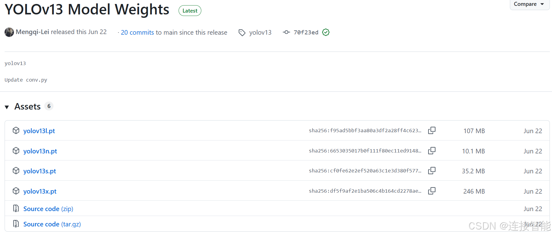
与之前的v11、v12不同,v13只有4种规模:n/s/l/x,缺少了middle规模,4种预训练模型下载地址如下:
https://github.com/iMoonLab/yolov13/releases/tag/yolov13
二、YOLOv13安装与使用
2.1安装过程
2.1.1环境要求
官方页面并没有提到相关的环境要求,但YOLOv13整体是在v12的基础上进行创新而成,因此需要使用flash_attn软件包或者scaled_dot_product_attention软件包,那么就要求pytorch版本是2.x系列,1.x系列无法使用YOLOv12、v13。
python版本最好使用较新的版本,例如3.12系列及以上。
2.1.2安装步骤
推荐读者不必按照官方github页面上的安装教程进行安装,而是参照如下安装步骤进行安装:
(1)下载源代码到本地
使用如下命令:
bash
git clone https://github.com/iMoonLab/yolov13.git(2)flash_attn软件包安装
flash_attn软件包并不是必选的,也可以不安装,如果需要安装,可参考本博客另一篇文章:YOLOv12模型安装及原理和代码解析
(3)检查缺少的其他依赖包
一般如果是新配置的运行环境,那么可能会提示缺少:yaml、matplotlib、requests、pandas、seaborn、polars、scipy等依赖包,读者可先检查是否安装了这些软件包,也可在首次调用YOLOv13进行训练时,根据提示安装对应的软件包即可。
(4)Arial字体文件与预训练权重下载
在首次调用YOLOv13进行训练之前,会进行Arial字体文件、预训练权重下载,如果网络不好的情况下建议手动下载,然后:
- 预训练权重放在训练代码同目录;
- Arial字体文件根据提示放在对应的目录,例如linux系统中会提示:
bash
Downloading https://ultralytics.com/assets/Arial.ttf to '/root/.config/yolov13/Arial.ttf'...2.2训练代码
下面给出了一个只指定了几个超参数的简单训练代码,供读者参考:
python
from ultralytics import YOLO

if __name__ == '__main__':
	model = YOLO('yolov13n.yaml')

	# Train the model
	results = model.train(
	  data='coco.yaml',
	  epochs=600,
	  batch=256,
	  imgsz=640,
	  optimizer='SGD',
	  scale=0.5,  # S:0.9; L:0.9; X:0.9
	  mosaic=1.0,
	  mixup=0.0,  # S:0.05; L:0.15; X:0.2
	  copy_paste=0.1,  # S:0.15; L:0.5; X:0.6
	  device="0",
	)
上述代码指定:使用sgd优化器,批次大小256,图像统一调整到640×640,训练600轮。
需要注意的是其中yolov13n.yaml文件其实是yolov13.yaml文件,n是指定使用文件中的哪一种规模,文件位于yolov13\ultralytics\cfg\models\v13,内容如下:
xml
nc: 80 # number of classes
scales: # model compound scaling constants, i.e. 'model=yolov13n.yaml' will call yolov13.yaml with scale 'n'
  # [depth, width, max_channels]
  n: [0.50, 0.25, 1024]   # Nano
  s: [0.50, 0.50, 1024]   # Small
  l: [1.00, 1.00, 512]    # Large
  x: [1.00, 1.50, 512]    # Extra Large

backbone:
  # [from, repeats, module, args]
  - [-1, 1, Conv,  [64, 3, 2]] # 0-P1/2
  - [-1, 1, Conv,  [128, 3, 2, 1, 2]] # 1-P2/4
  - [-1, 2, DSC3k2,  [256, False, 0.25]]
  - [-1, 1, Conv,  [256, 3, 2, 1, 4]] # 3-P3/8
  - [-1, 2, DSC3k2,  [512, False, 0.25]]
  - [-1, 1, DSConv,  [512, 3, 2]] # 5-P4/16
  - [-1, 4, A2C2f, [512, True, 4]]
  - [-1, 1, DSConv,  [1024, 3, 2]] # 7-P5/32
  - [-1, 4, A2C2f, [1024, True, 1]] # 8

head:
  - [[4, 6, 8], 2, HyperACE, [512, 8, True, True, 0.5, 1, "both"]]
  - [-1, 1, nn.Upsample, [None, 2, "nearest"]]
  - [ 9, 1, DownsampleConv, []]
  - [[6, 9], 1, FullPAD_Tunnel, []]  #12
  - [[4, 10], 1, FullPAD_Tunnel, []]  #13
  - [[8, 11], 1, FullPAD_Tunnel, []] #14

  - [-1, 1, nn.Upsample, [None, 2, "nearest"]]
  - [[-1, 12], 1, Concat, [1]] # cat backbone P4
  - [-1, 2, DSC3k2, [512, True]] # 17
  - [[-1, 9], 1, FullPAD_Tunnel, []]  #18

  - [17, 1, nn.Upsample, [None, 2, "nearest"]]
  - [[-1, 13], 1, Concat, [1]] # cat backbone P3
  - [-1, 2, DSC3k2, [256, True]] # 21
  - [10, 1, Conv, [256, 1, 1]]
  - [[21, 22], 1, FullPAD_Tunnel, []]  #23

  - [-1, 1, Conv, [256, 3, 2]]
  - [[-1, 18], 1, Concat, [1]] # cat head P4
  - [-1, 2, DSC3k2, [512, True]] # 26
  - [[-1, 9], 1, FullPAD_Tunnel, []]

  - [26, 1, Conv, [512, 3, 2]]
  - [[-1, 14], 1, Concat, [1]] # cat head P5
  - [-1, 2, DSC3k2, [1024,True]] # 30 (P5/32-large)
  - [[-1, 11], 1, FullPAD_Tunnel, []]

  - [[23, 27, 31], 1, Detect, [nc]] # Detect(P3, P4, P5)
coco.yaml设置了使用数据集的路径,文件位于yolov13\ultralytics\cfg\datasets\coco.yaml,如果使用其他数据集,要进行修改,原始内容如下:
xml
# Ultralytics 🚀 AGPL-3.0 License - https://ultralytics.com/license

# COCO 2017 dataset https://cocodataset.org by Microsoft
# Documentation: https://docs.ultralytics.com/datasets/detect/coco/
# Example usage: yolo train data=coco.yaml
# parent
# ├── ultralytics
# └── datasets
#     └── coco  ← downloads here (20.1 GB)

# Train/val/test sets as 1) dir: path/to/imgs, 2) file: path/to/imgs.txt, or 3) list: [path/to/imgs1, path/to/imgs2, ..]
path: ..datasets/coco # dataset root dir
train: train2017.txt # train images (relative to 'path') 118287 images
val: val2017.txt # val images (relative to 'path') 5000 images
test: test-dev2017.txt # 20288 of 40670 images, submit to https://competitions.codalab.org/competitions/20794

# Classes
names:
  0: person
  1: bicycle
  2: car
  ...
  78: hair drier
  79: toothbrush

# Download script/URL (optional)
download: |
  from ultralytics.utils.downloads import download
  from pathlib import Path

  # Download labels
  segments = True  # segment or box labels
  dir = Path(yaml['path'])  # dataset root dir
  url = 'https://github.com/ultralytics/assets/releases/download/v0.0.0/'
  urls = [url + ('coco2017labels-segments.zip' if segments else 'coco2017labels.zip')]  # labels
  download(urls, dir=dir.parent)
  # Download data
  urls = ['http://images.cocodataset.org/zips/train2017.zip',  # 19G, 118k images
          'http://images.cocodataset.org/zips/val2017.zip',  # 1G, 5k images
          'http://images.cocodataset.org/zips/test2017.zip']  # 7G, 41k images (optional)
  download(urls, dir=dir / 'images', threads=3)
2.3评估代码
简单的评估代码如下:
python
from ultralytics import YOLO

if __name__ == '__main__':
    model = YOLO("best.pt")

    metrics = model.val(
        data="custom.yaml",
        imgsz=640,
        batch=256,
        plots=True
    )
上述代码指定:需要评估的模型路径,然后选择数据集的配置文件,将图像统一调整大小至640×640,批次大小256,评估结果绘制图片。
三、YOLOv13原理和代码解析
3.1概述
论文中提到,以卷积为主的YOLOv11和以注意力机制为主的YOLOv12,他们的局限性在于只进行了局部信息聚合以及像素或像素块间的两两之间的相关性建模,缺少捕捉全局之间的多对多的高阶相关性建模,因此造成了在复杂场景中的检测性能不佳。
YOLOv13通过引入
- 基于超图的自适应相关性增强机制(Hypergraph-based Adaptive Correlation Enhancement,HyperACE),能够捕捉潜在的高阶相关性;
- 基于HyperACE的全流水线聚合与分发范式(Full-Pipeline Aggregation-and-Distribution,FullPAD),改善细粒度的信息流动和协同表征;
- 深度可分离卷积替换掉原始的大核卷积,从而降低计算复杂度。
以上三个核心改进,来提高YOLO模型的识别精度且保持实时性。
3.2HyperACE模块
3.2.1超图(Hypergraph)概念
超图与传统的图区别之处在于,传统的图中一条边仅可以连接两个顶点,而超图中的超边可以连接多个顶点,因此可以对多个顶点之间的相关性建模。
一些研究已经证明,建立多像素间的高阶相关性对于视觉检测任务是有所帮助的。
3.2.2自适应超图计算(Adaptive Hypergraph Computation)
传统的超图建模是使用认为设定的阈值建立超边,而自适应超图可以自适应学习每个顶点对于超边的参与度进行建模。
自适应超图计算分为以下两个部分。
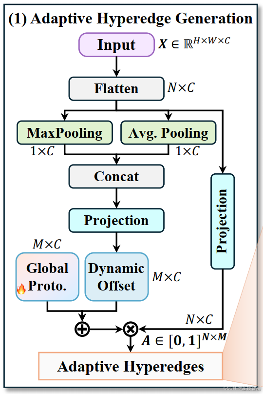
3.2.2.1自适应超边生成
超图中的顶点是输入的像素或特征向量的集合,设数量为N,通道数为C,设定产生的超边数量为M。
超边生成步骤如下:
- 第一步先展平为N×C,分别进行全局平均池化和最大池化操作,然后拼接在一起产生全局上下文向量,记为fctx,维度是2C;
- fctx经过一个映射层调整通道数,产生超边的全局偏移向量,产生维度为M×C;
- 生成一个可学习的超边基础原型P,与上一步中的偏移向量相加,得到相加后的超边原型;
- 这个超边原型与原始输入的顶点像素向量计算相似度,最终再归一化,生成最终的参与度矩阵A。
超边生成的最终结果是生成一个参与度矩阵,类似于每个顶点隶属于每个超边的隶属度。为避免增加理解难度,第四步中还有一个多头机制此处省略掉。
实现的源码如下:
python
class AdaHyperedgeGen(nn.Module):
    """
    Generates an adaptive hyperedge participation matrix from a set of vertex features.

    This module implements the Adaptive Hyperedge Generation mechanism. It generates dynamic hyperedge prototypes
    based on the global context of the input nodes and calculates a continuous participation matrix (A)
    that defines the relationship between each vertex and each hyperedge.

    Attributes:
        node_dim (int): The feature dimension of each input node.
        num_hyperedges (int): The number of hyperedges to generate.
        num_heads (int, optional): The number of attention heads for multi-head similarity calculation. Defaults to 4.
        dropout (float, optional): The dropout rate applied to the logits. Defaults to 0.1.
        context (str, optional): The type of global context to use ('mean', 'max', or 'both'). Defaults to "both".

    Methods:
        forward: Takes a batch of vertex features and returns the participation matrix A.

    Examples:
        >>> import torch
        >>> model = AdaHyperedgeGen(node_dim=64, num_hyperedges=16, num_heads=4)
        >>> x = torch.randn(2, 100, 64)  # (Batch, Num_Nodes, Node_Dim)
        >>> A = model(x)
        >>> print(A.shape)
        torch.Size([2, 100, 16])
    """
    def __init__(self, node_dim, num_hyperedges, num_heads=4, dropout=0.1, context="both"):
        super().__init__()
        self.num_heads = num_heads
        self.num_hyperedges = num_hyperedges
        self.head_dim = node_dim // num_heads
        self.context = context

        self.prototype_base = nn.Parameter(torch.Tensor(num_hyperedges, node_dim))
        nn.init.xavier_uniform_(self.prototype_base)
        if context in ("mean", "max"):
            self.context_net = nn.Linear(node_dim, num_hyperedges * node_dim)
        elif context == "both":
            self.context_net = nn.Linear(2*node_dim, num_hyperedges * node_dim)
        else:
            raise ValueError(
                f"Unsupported context '{context}'. "
                "Expected one of: 'mean', 'max', 'both'."
            )

        self.pre_head_proj = nn.Linear(node_dim, node_dim)

        self.dropout = nn.Dropout(dropout)
        self.scaling = math.sqrt(self.head_dim)

    def forward(self, X):
        B, N, D = X.shape
        if self.context == "mean":
            context_cat = X.mean(dim=1)
        elif self.context == "max":
            context_cat, _ = X.max(dim=1)
        else:
            avg_context = X.mean(dim=1)
            max_context, _ = X.max(dim=1)
            context_cat = torch.cat([avg_context, max_context], dim=-1)
        prototype_offsets = self.context_net(context_cat).view(B, self.num_hyperedges, D)
        prototypes = self.prototype_base.unsqueeze(0) + prototype_offsets

        X_proj = self.pre_head_proj(X)
        X_heads = X_proj.view(B, N, self.num_heads, self.head_dim).transpose(1, 2)
        proto_heads = prototypes.view(B, self.num_hyperedges, self.num_heads, self.head_dim).permute(0, 2, 1, 3)

        X_heads_flat = X_heads.reshape(B * self.num_heads, N, self.head_dim)
        proto_heads_flat = proto_heads.reshape(B * self.num_heads, self.num_hyperedges, self.head_dim).transpose(1, 2)

        logits = torch.bmm(X_heads_flat, proto_heads_flat) / self.scaling
        logits = logits.view(B, self.num_heads, N, self.num_hyperedges).mean(dim=1)

        logits = self.dropout(logits)

        return F.softmax(logits, dim=1)
代码逻辑基本符合上述实现步骤,其中超边基础原型是使用torch.Tensor产生的一个初始张量。
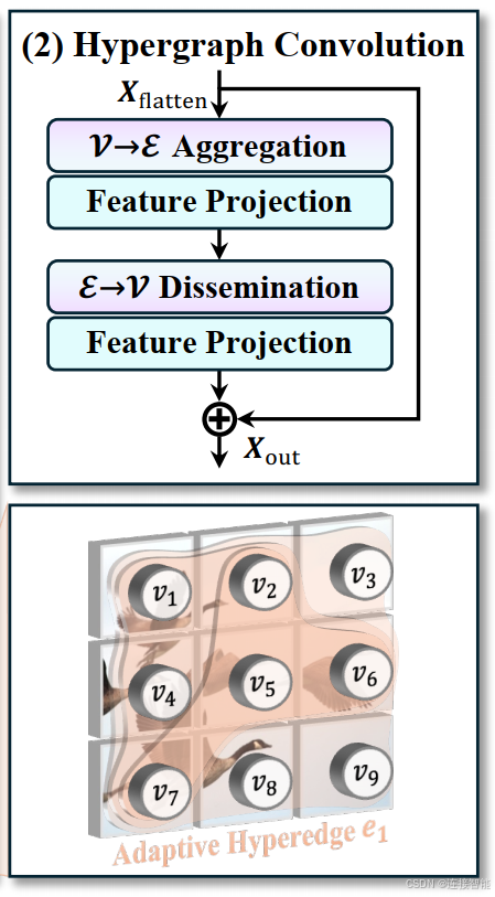
3.2.2.2超图卷积
超图卷积,这一操作是为了实现特征聚合与增强,实现过程并不复杂:
- 上一小节产生的参与度矩阵与原始输入的像素进行相乘,然后进行映射及激活,产生一个超边特征向量;
- 对产生的超边特征向量执行与第一步相同的操作,与参与度矩阵相乘,然后进行映射及激活,产生与原始输入维度相同的得到增强的特征向量。
实现代码如下:
python
class AdaHGConv(nn.Module):
    """
    Performs the adaptive hypergraph convolution.

    This module contains the two-stage message passing process of hypergraph convolution:
    1. Generates an adaptive participation matrix using AdaHyperedgeGen.
    2. Aggregates vertex features into hyperedge features (vertex-to-edge).
    3. Disseminates hyperedge features back to update vertex features (edge-to-vertex).
    A residual connection is added to the final output.

    Attributes:
        embed_dim (int): The feature dimension of the vertices.
        num_hyperedges (int, optional): The number of hyperedges for the internal generator. Defaults to 16.
        num_heads (int, optional): The number of attention heads for the internal generator. Defaults to 4.
        dropout (float, optional): The dropout rate for the internal generator. Defaults to 0.1.
        context (str, optional): The context type for the internal generator. Defaults to "both".

    Methods:
        forward: Performs the adaptive hypergraph convolution on a batch of vertex features.

    Examples:
        >>> import torch
        >>> model = AdaHGConv(embed_dim=128, num_hyperedges=16, num_heads=8)
        >>> x = torch.randn(2, 256, 128) # (Batch, Num_Nodes, Dim)
        >>> output = model(x)
        >>> print(output.shape)
        torch.Size([2, 256, 128])
    """
    def __init__(self, embed_dim, num_hyperedges=16, num_heads=4, dropout=0.1, context="both"):
        super().__init__()
        self.edge_generator = AdaHyperedgeGen(embed_dim, num_hyperedges, num_heads, dropout, context)
        self.edge_proj = nn.Sequential(
            nn.Linear(embed_dim, embed_dim ),
            nn.GELU()
        )
        self.node_proj = nn.Sequential(
            nn.Linear(embed_dim, embed_dim ),
            nn.GELU()
        )

    def forward(self, X):
        A = self.edge_generator(X)

        He = torch.bmm(A.transpose(1, 2), X)
        He = self.edge_proj(He)

        X_new = torch.bmm(A, He)
        X_new = self.node_proj(X_new)

        return X_new + X
代码中,最终输出是原始输入与增强后的输入相加的结果,这一点论文中似乎没有提到。
3.2.2.3整体实现代码
自适应超图计算具体是通过依次执行上述两小节来实现,整体实现代码如下:
python
class AdaHGComputation(nn.Module):
"""
A wrapper module for applying adaptive hypergraph convolution to 4D feature maps.
This class makes the hypergraph convolution compatible with standard CNN architectures. It flattens a
4D input tensor (B, C, H, W) into a sequence of vertices (tokens), applies the AdaHGConv layer to
model high-order correlations, and then reshapes the output back into a 4D tensor.
Attributes:
embed_dim (int): The feature dimension of the vertices (equivalent to input channels C).
num_hyperedges (int, optional): The number of hyperedges for the underlying AdaHGConv. Defaults to 16.
num_heads (int, optional): The number of attention heads for the underlying AdaHGConv. Defaults to 8.
dropout (float, optional): The dropout rate for the underlying AdaHGConv. Defaults to 0.1.
context (str, optional): The context type for the underlying AdaHGConv. Defaults to "both".
Methods:
forward: Processes a 4D feature map through the adaptive hypergraph computation layer.
Examples:
>>> import torch
>>> model = AdaHGComputation(embed_dim=64, num_hyperedges=8, num_heads=4)
>>> x = torch.randn(2, 64, 32, 32) # (B, C, H, W)
>>> output = model(x)
>>> print(output.shape)
torch.Size([2, 64, 32, 32])
"""
def __init__(self, embed_dim, num_hyperedges=16, num_heads=8, dropout=0.1, context="both"):
super().__init__()
self.embed_dim = embed_dim
self.hgnn = AdaHGConv(
embed_dim=embed_dim,
num_hyperedges=num_hyperedges,
num_heads=num_heads,
dropout=dropout,
context=context
)
def forward(self, x):
B, C, H, W = x.shape
tokens = x.flatten(2).transpose(1, 2)
tokens = self.hgnn(tokens)
x_out = tokens.transpose(1, 2).view(B, C, H, W)
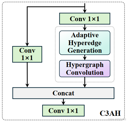
return x_out 3.2.3自适应高阶相关性建模
自适应高阶相关性建模是通过C3AH模块实现的,模块结构类似于YOLO模型的CSP模块,如下图所示:
实现过程较为简单,代码如下:
python
class C3AH(nn.Module):
    """
    A CSP-style block integrating Adaptive Hypergraph Computation (C3AH).

    The input feature map is split into two paths.
    One path is processed by the AdaHGComputation module to model high-order correlations, while the other
    serves as a shortcut. The outputs are then concatenated to fuse features.

    Attributes:
        c1 (int): Number of input channels.
        c2 (int): Number of output channels.
        e (float, optional): Expansion ratio for the hidden channels. Defaults to 1.0.
        num_hyperedges (int, optional): The number of hyperedges for the internal AdaHGComputation. Defaults to 8.
        context (str, optional): The context type for the internal AdaHGComputation. Defaults to "both".

    Methods:
        forward: Performs a forward pass through the C3AH module.

    Examples:
        >>> import torch
        >>> model = C3AH(c1=64, c2=128, num_hyperedges=8)
        >>> x = torch.randn(2, 64, 32, 32)
        >>> output = model(x)
        >>> print(output.shape)
        torch.Size([2, 128, 32, 32])
    """
    def __init__(self, c1, c2, e=1.0, num_hyperedges=8, context="both"):
        super().__init__()
        c_ = int(c2 * e)
        assert c_ % 16 == 0, "Dimension of AdaHGComputation should be a multiple of 16."
        num_heads = c_ // 16
        self.cv1 = Conv(c1, c_, 1, 1)
        self.cv2 = Conv(c1, c_, 1, 1)
        self.m = AdaHGComputation(embed_dim=c_,
                          num_hyperedges=num_hyperedges,
                          num_heads=num_heads,
                          dropout=0.1,
                          context=context)
        self.cv3 = Conv(2 * c_, c2, 1)

    def forward(self, x):
        return self.cv3(torch.cat((self.m(self.cv1(x)), self.cv2(x)), 1))
代码中的AdaHGComputation即为上一节的自适应超图计算。
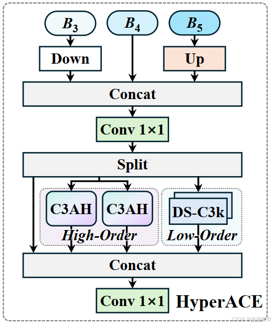
3.2.4HyperACE结构
HyperACE接收Backbone输出的B3、B4和B5三个尺度的特征,然后分别进行高阶相关性增强和低阶相关性增强,最终将高阶、低阶以及未增强的原始特征通过一个1×1卷积融合到一起,输出一个高阶与低阶感知互补的特征图。
其中高阶相关性建模使用C3AH模块实现,低阶相关性建模使用的DSC3k模块实现,结构如下图:
实现代码如下:
python
class FuseModule(nn.Module):
    """
    A module to fuse multi-scale features for the HyperACE block.

    This module takes a list of three feature maps from different scales, aligns them to a common
    spatial resolution by downsampling the first and upsampling the third, and then concatenates
    and fuses them with a convolution layer.

    Attributes:
        c_in (int): The number of channels of the input feature maps.
        channel_adjust (bool): Whether to adjust the channel count of the concatenated features.

    Methods:
        forward: Fuses a list of three multi-scale feature maps.

    Examples:
        >>> import torch
        >>> model = FuseModule(c_in=64, channel_adjust=False)
        >>> # Input is a list of features from different backbone stages
        >>> x_list = [torch.randn(2, 64, 64, 64), torch.randn(2, 64, 32, 32), torch.randn(2, 64, 16, 16)]
        >>> output = model(x_list)
        >>> print(output.shape)
        torch.Size([2, 64, 32, 32])
    """
    def __init__(self, c_in, channel_adjust):
        super(FuseModule, self).__init__()
        self.downsample = nn.AvgPool2d(kernel_size=2)
        self.upsample = nn.Upsample(scale_factor=2, mode='nearest')
        if channel_adjust:
            self.conv_out = Conv(4 * c_in, c_in, 1)
        else:
            self.conv_out = Conv(3 * c_in, c_in, 1)

    def forward(self, x):
        x1_ds = self.downsample(x[0])
        x3_up = self.upsample(x[2])
        x_cat = torch.cat([x1_ds, x[1], x3_up], dim=1)
        out = self.conv_out(x_cat)
        return out

class HyperACE(nn.Module):
    """
    Hypergraph-based Adaptive Correlation Enhancement (HyperACE).

    This is the core module of YOLOv13, designed to model both global high-order correlations and
    local low-order correlations. It first fuses multi-scale features, then processes them through parallel
    branches: two C3AH branches for high-order modeling and a lightweight DSConv-based branch for
    low-order feature extraction.

    Attributes:
        c1 (int): Number of input channels for the fuse module.
        c2 (int): Number of output channels for the entire block.
        n (int, optional): Number of blocks in the low-order branch. Defaults to 1.
        num_hyperedges (int, optional): Number of hyperedges for the C3AH branches. Defaults to 8.
        dsc3k (bool, optional): If True, use DSC3k in the low-order branch; otherwise, use DSBottleneck. Defaults to True.
        shortcut (bool, optional): Whether to use shortcuts in the low-order branch. Defaults to False.
        e1 (float, optional): Expansion ratio for the main hidden channels. Defaults to 0.5.
        e2 (float, optional): Expansion ratio within the C3AH branches. Defaults to 1.
        context (str, optional): Context type for C3AH branches. Defaults to "both".
        channel_adjust (bool, optional): Passed to FuseModule for channel configuration. Defaults to True.

    Methods:
        forward: Performs a forward pass through the HyperACE module.

    Examples:
        >>> import torch
        >>> model = HyperACE(c1=64, c2=256, n=1, num_hyperedges=8)
        >>> x_list = [torch.randn(2, 64, 64, 64), torch.randn(2, 64, 32, 32), torch.randn(2, 64, 16, 16)]
        >>> output = model(x_list)
        >>> print(output.shape)
        torch.Size([2, 256, 32, 32])
    """
    def __init__(self, c1, c2, n=1, num_hyperedges=8, dsc3k=True, shortcut=False, e1=0.5, e2=1, context="both", channel_adjust=True):
        super().__init__()
        self.c = int(c2 * e1)
        self.cv1 = Conv(c1, 3 * self.c, 1, 1)
        self.cv2 = Conv((4 + n) * self.c, c2, 1)
        self.m = nn.ModuleList(
            DSC3k(self.c, self.c, 2, shortcut, k1=3, k2=7) if dsc3k else DSBottleneck(self.c, self.c, shortcut=shortcut) for _ in range(n)
        )
        self.fuse = FuseModule(c1, channel_adjust)
        self.branch1 = C3AH(self.c, self.c, e2, num_hyperedges, context)
        self.branch2 = C3AH(self.c, self.c, e2, num_hyperedges, context)

    def forward(self, X):
        x = self.fuse(X)
        y = list(self.cv1(x).chunk(3, 1))
        out1 = self.branch1(y[1])
        out2 = self.branch2(y[1])
        y.extend(m(y[-1]) for m in self.m)
        y[1] = out1
        y.append(out2)
        return self.cv2(torch.cat(y, 1))
3.3FullPAD范式
3.3.1原理
FullPAD范式是一种特征图的调配管理方式,它首先将backbone输出的B3, B4, B5特征图输入到HyperACE模块进行特征增强,然后将增强后的特征图调增尺度和通道数,最后乘以一个可学习的权重因子与任意特征图相加,起到增强原始特征图的作用。
FullPAD范式有3个通道,将增强的特征图传递到模型信息流水线上的7个位置,与相应的特征图相加,改善梯度传播和检测性能。
3.3.2实现代码
如上一节所述,FullPAD范式是一种特征图的分配模式,并不是单一的模块单元,所以它的实现主要是在模型结构中进行定义,源码中只有通道相关的实现代码如下:
python
class FullPAD_Tunnel(nn.Module):
    """
    A gated fusion module for the Full-Pipeline Aggregation-and-Distribution (FullPAD) paradigm.

    This module implements a gated residual connection used to fuse features. It takes two inputs: the original
    feature map and a correlation-enhanced feature map. It then computes `output = original + gate * enhanced`,
    where `gate` is a learnable scalar parameter that adaptively balances the contribution of the enhanced features.

    Methods:
        forward: Performs the gated fusion of two input feature maps.

    Examples:
        >>> import torch
        >>> model = FullPAD_Tunnel()
        >>> original_feature = torch.randn(2, 64, 32, 32)
        >>> enhanced_feature = torch.randn(2, 64, 32, 32)
        >>> output = model([original_feature, enhanced_feature])
        >>> print(output.shape)
        torch.Size([2, 64, 32, 32])
    """
    def __init__(self):
        super().__init__()
        self.gate = nn.Parameter(torch.tensor(0.0))
    def forward(self, x):
        out = x[0] + self.gate * x[1]
        return out
代码较为简单,其中gate即为可学习的权重因子。
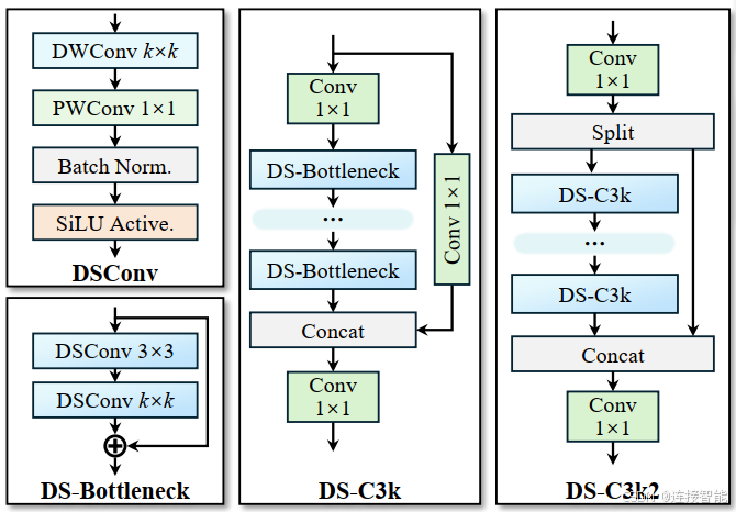
3.4DSC3k2模块
3.4.1原理
YOLOv13引入了超图必然会导致模型计算复杂度上升,所以需要使用深度可分离卷积来降低计算复杂度,因此将原有C3k2模块中的卷积替换为了DS卷积,提出了DSC3k2模块。
DSC3k2模块结构图如下,与C3k2模块结构基本一致:
3.4.2实现代码
实现代码如下:
python
class DSBottleneck(nn.Module):
    """
    An improved bottleneck block using depthwise separable convolutions (DSConv).

    This class implements a lightweight bottleneck module that replaces standard convolutions with depthwise
    separable convolutions to reduce parameters and computational cost.

    Attributes:
        c1 (int): Number of input channels.
        c2 (int): Number of output channels.
        shortcut (bool, optional): Whether to use a residual shortcut connection. The connection is only added if c1 == c2. Defaults to True.
        e (float, optional): Expansion ratio for the intermediate channels. Defaults to 0.5.
        k1 (int, optional): Kernel size for the first DSConv layer. Defaults to 3.
        k2 (int, optional): Kernel size for the second DSConv layer. Defaults to 5.
        d2 (int, optional): Dilation for the second DSConv layer. Defaults to 1.

    Methods:
        forward: Performs a forward pass through the DSBottleneck module.

    Examples:
        >>> import torch
        >>> model = DSBottleneck(c1=64, c2=64, shortcut=True)
        >>> x = torch.randn(2, 64, 32, 32)
        >>> output = model(x)
        >>> print(output.shape)
        torch.Size([2, 64, 32, 32])
    """
    def __init__(self, c1, c2, shortcut=True, e=0.5, k1=3, k2=5, d2=1):
        super().__init__()
        c_ = int(c2 * e)
        self.cv1 = DSConv(c1, c_, k1, s=1, p=None, d=1)
        self.cv2 = DSConv(c_, c2, k2, s=1, p=None, d=d2)
        self.add = shortcut and c1 == c2

    def forward(self, x):
        y = self.cv2(self.cv1(x))
        return x + y if self.add else y


class DSC3k(C3):
    """
    An improved C3k module using DSBottleneck blocks for lightweight feature extraction.

    This class extends the C3 module by replacing its standard bottleneck blocks with DSBottleneck blocks,
    which use depthwise separable convolutions.

    Attributes:
        c1 (int): Number of input channels.
        c2 (int): Number of output channels.
        n (int, optional): Number of DSBottleneck blocks to stack. Defaults to 1.
        shortcut (bool, optional): Whether to use shortcut connections within the DSBottlenecks. Defaults to True.
        g (int, optional): Number of groups for grouped convolution (passed to parent C3). Defaults to 1.
        e (float, optional): Expansion ratio for the C3 module's hidden channels. Defaults to 0.5.
        k1 (int, optional): Kernel size for the first DSConv in each DSBottleneck. Defaults to 3.
        k2 (int, optional): Kernel size for the second DSConv in each DSBottleneck. Defaults to 5.
        d2 (int, optional): Dilation for the second DSConv in each DSBottleneck. Defaults to 1.

    Methods:
        forward: Performs a forward pass through the DSC3k module (inherited from C3).

    Examples:
        >>> import torch
        >>> model = DSC3k(c1=128, c2=128, n=2, k1=3, k2=7)
        >>> x = torch.randn(2, 128, 64, 64)
        >>> output = model(x)
        >>> print(output.shape)
        torch.Size([2, 128, 64, 64])
    """
    def __init__(
        self,
        c1,
        c2,
        n=1,
        shortcut=True,
        g=1,
        e=0.5,
        k1=3,
        k2=5,
        d2=1
    ):
        super().__init__(c1, c2, n, shortcut, g, e)
        c_ = int(c2 * e)

        self.m = nn.Sequential(
            *(
                DSBottleneck(
                    c_, c_,
                    shortcut=shortcut,
                    e=1.0,
                    k1=k1,
                    k2=k2,
                    d2=d2
                )
                for _ in range(n)
            )
        )

class DSC3k2(C2f):
    """
    An improved C3k2 module that uses lightweight depthwise separable convolution blocks.

    This class redesigns C3k2 module, replacing its internal processing blocks with either DSBottleneck
    or DSC3k modules.

    Attributes:
        c1 (int): Number of input channels.
        c2 (int): Number of output channels.
        n (int, optional): Number of internal processing blocks to stack. Defaults to 1.
        dsc3k (bool, optional): If True, use DSC3k as the internal block. If False, use DSBottleneck. Defaults to False.
        e (float, optional): Expansion ratio for the C2f module's hidden channels. Defaults to 0.5.
        g (int, optional): Number of groups for grouped convolution (passed to parent C2f). Defaults to 1.
        shortcut (bool, optional): Whether to use shortcut connections in the internal blocks. Defaults to True.
        k1 (int, optional): Kernel size for the first DSConv in internal blocks. Defaults to 3.
        k2 (int, optional): Kernel size for the second DSConv in internal blocks. Defaults to 7.
        d2 (int, optional): Dilation for the second DSConv in internal blocks. Defaults to 1.

    Methods:
        forward: Performs a forward pass through the DSC3k2 module (inherited from C2f).

    Examples:
        >>> import torch
        >>> # Using DSBottleneck as internal block
        >>> model1 = DSC3k2(c1=64, c2=64, n=2, dsc3k=False)
        >>> x = torch.randn(2, 64, 128, 128)
        >>> output1 = model1(x)
        >>> print(f"With DSBottleneck: {output1.shape}")
        With DSBottleneck: torch.Size([2, 64, 128, 128])
        >>> # Using DSC3k as internal block
        >>> model2 = DSC3k2(c1=64, c2=64, n=1, dsc3k=True)
        >>> output2 = model2(x)
        >>> print(f"With DSC3k: {output2.shape}")
        With DSC3k: torch.Size([2, 64, 128, 128])
    """
    def __init__(
        self,
        c1,
        c2,
        n=1,
        dsc3k=False,
        e=0.5,
        g=1,
        shortcut=True,
        k1=3,
        k2=7,
        d2=1
    ):
        super().__init__(c1, c2, n, shortcut, g, e)
        if dsc3k:
            self.m = nn.ModuleList(
                DSC3k(
                    self.c, self.c,
                    n=2,
                    shortcut=shortcut,
                    g=g,
                    e=1.0,
                    k1=k1,
                    k2=k2,
                    d2=d2
                )
                for _ in range(n)
            )
        else:
            self.m = nn.ModuleList(
                DSBottleneck(
                    self.c, self.c,
                    shortcut=shortcut,
                    e=1.0,
                    k1=k1,
                    k2=k2,
                    d2=d2
                )
                for _ in range(n)
            )
实现代码与原有的C3k2模块基本一致,只是将原始Bottleneck类中的Conv替换为了DSBottleneck类中的DSConv。
3.5整体结构
3.5.1结构分析
整体结构如图:
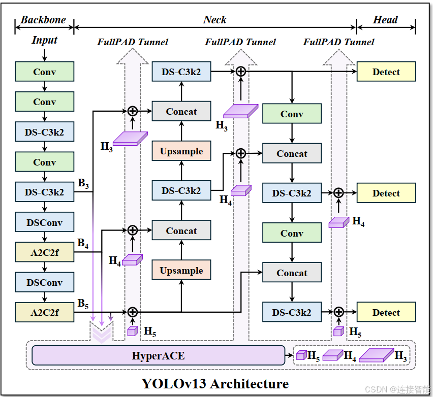
从结构图可看出:
- YOLOv13整体延续了backbone-neck-head这一三段式结构,而结构图中的A2C2f模块表明v13继承了v12的注意力机制;
- FullPAD范式将B3、B4和B5输入到HyperACE模块产生增强的H4,分别对H4上、下采样得到H3与H5;
- 然后分别将H3、H4和H5传送到结构图中的7个位置与相应的特征图相加。
3.5.2结构定义代码
YOLOv13模型结构同样是在yaml文件中进行定义,yolov13.yaml文件内容如下:
xml
nc: 80 # number of classes
scales: # model compound scaling constants, i.e. 'model=yolov13n.yaml' will call yolov13.yaml with scale 'n'
  # [depth, width, max_channels]
  n: [0.50, 0.25, 1024]   # Nano
  s: [0.50, 0.50, 1024]   # Small
  l: [1.00, 1.00, 512]    # Large
  x: [1.00, 1.50, 512]    # Extra Large

backbone:
  # [from, repeats, module, args]
  - [-1, 1, Conv,  [64, 3, 2]] # 0-P1/2
  - [-1, 1, Conv,  [128, 3, 2, 1, 2]] # 1-P2/4
  - [-1, 2, DSC3k2,  [256, False, 0.25]]
  - [-1, 1, Conv,  [256, 3, 2, 1, 4]] # 3-P3/8
  - [-1, 2, DSC3k2,  [512, False, 0.25]]
  - [-1, 1, DSConv,  [512, 3, 2]] # 5-P4/16
  - [-1, 4, A2C2f, [512, True, 4]]
  - [-1, 1, DSConv,  [1024, 3, 2]] # 7-P5/32
  - [-1, 4, A2C2f, [1024, True, 1]] # 8

head:
  - [[4, 6, 8], 2, HyperACE, [512, 8, True, True, 0.5, 1, "both"]]
  - [-1, 1, nn.Upsample, [None, 2, "nearest"]]
  - [ 9, 1, DownsampleConv, []]
  - [[6, 9], 1, FullPAD_Tunnel, []]  #12
  - [[4, 10], 1, FullPAD_Tunnel, []]  #13
  - [[8, 11], 1, FullPAD_Tunnel, []] #14

  - [-1, 1, nn.Upsample, [None, 2, "nearest"]]
  - [[-1, 12], 1, Concat, [1]] # cat backbone P4
  - [-1, 2, DSC3k2, [512, True]] # 17
  - [[-1, 9], 1, FullPAD_Tunnel, []]  #18

  - [17, 1, nn.Upsample, [None, 2, "nearest"]]
  - [[-1, 13], 1, Concat, [1]] # cat backbone P3
  - [-1, 2, DSC3k2, [256, True]] # 21
  - [10, 1, Conv, [256, 1, 1]]
  - [[21, 22], 1, FullPAD_Tunnel, []]  #23

  - [-1, 1, Conv, [256, 3, 2]]
  - [[-1, 18], 1, Concat, [1]] # cat head P4
  - [-1, 2, DSC3k2, [512, True]] # 26
  - [[-1, 9], 1, FullPAD_Tunnel, []]

  - [26, 1, Conv, [512, 3, 2]]
  - [[-1, 14], 1, Concat, [1]] # cat head P5
  - [-1, 2, DSC3k2, [1024,True]] # 30 (P5/32-large)
  - [[-1, 11], 1, FullPAD_Tunnel, []]

  - [[23, 27, 31], 1, Detect, [nc]] # Detect(P3, P4, P5)
3.5.3yaml文件解析规则
Ultralytics系列的模型yaml文件,每一层都遵循同一结构:from, number, module, args。
| 字段 | 含义 |
|---|---|
| from | 输入来源(上一层或指定层索引) |
| number | 该模块重复的次数(depth scaling 前) |
| module | 使用的模块 |
| args | 模块的构造参数 |
以- \[4, 6, 8, 2, HyperACE, 512, 8, True, True, 0.5, 1, "both"]为例:
- 输入为4, 6, 8,即第4、6、8层的输出,就是B3、B4和B5;
- 2, HyperACE,重复使用2次HyperACE模块;
- 512, 8, True, True, 0.5, 1, "both",即为HyperACE模块的参数。