Softplus Function - Derivatives and Gradients (导数和梯度)

Softplus Function - Derivatives and Gradients {导数和梯度}

• [1. Softplus Function](#1. Softplus Function)
• • [1.1. Parameters](#1.1. Parameters)
  • [1.2. Shape](#1.2. Shape)
• [2. Softplus Function - Derivatives and Gradients (导数和梯度)](#2. Softplus Function - Derivatives and Gradients (导数和梯度))
• • [2.1. PyTorch `torch.nn.Softplus(beta=1.0, threshold=20.0)`](#2.1. PyTorch torch.nn.Softplus(beta=1.0, threshold=20.0))
  • [2.2. PyTorch `torch.nn.Softplus(beta=1.0, threshold=20.0)`](#2.2. PyTorch torch.nn.Softplus(beta=1.0, threshold=20.0))
  • [2.3. Python Softplus Function](#2.3. Python Softplus Function)
  • [2.4. Python Softplus Function](#2.4. Python Softplus Function)
• References

1. Softplus Function

class torch.nn.Softplus(beta=1.0, threshold=20.0)
https://docs.pytorch.org/docs/stable/generated/torch.nn.Softplus.html

torch.nn.functional.softplus(input, beta=1, threshold=20) -> Tensor
https://docs.pytorch.org/docs/stable/generated/torch.nn.functional.softplus.html

https://github.com/pytorch/pytorch/blob/v2.9.1/torch/nn/modules/activation.py

class torch.nn.Softplus(beta=1.0, threshold=20.0)

Applies the Softplus function element-wise.

SoftPlus is a smooth approximation to the ReLU function and can be used to constrain the output of a machine to always be positive.

For numerical stability the implementation reverts to the linear function when i n p u t × β > t h r e s h o l d input \times \beta > threshold input×β>threshold.

Calculating e x p ( x ) exp(x) exp(x) directly for x > 700 x>700 x>700 causes overflow in standard 64-bit floats.

By setting a threshold (typically 20), we treat the function as linear for very large inputs, as ln ⁡ ( 1 + e 20 ) ≈ 20 \ln (1+e^{20})\approx 20 ln(1+e20)≈20. Standard libraries like PyTorch and TensorFlow use a threshold (typically 20) to switch to a linear function ( f ( x ) ≈ x f(x)\approx x f(x)≈x) for large inputs to ensure stability.

revert [rɪˈvɜː(r)t]
v. 回复
n. 归属；恢复原来信仰的人

In PyTorch, the torch.nn.Softplus module or torch.nn.functional.softplus function includes an adjustable parameter β \beta β and a threshold for numerical stability.

The definition of the Softplus function:

Softplus ( x ) = 1 β ∗ log ⁡ ( 1 + exp ⁡ ( β ∗ x ) ) = 1 β ∗ log ⁡ e ( 1 + e ( β ∗ x ) ) \begin{aligned} \text{Softplus}(x) &= \frac{1}{\beta} * \log(1 + \exp(\beta * x)) \\ &= \frac{1}{\beta} * \log_{e}(1 + e^{(\beta * x)}) \\ \end{aligned} Softplus(x)=β1∗log(1+exp(β∗x))=β1∗loge(1+e(β∗x))

The derivative of the Softplus function:

d y d x = f ′ ( x ) = 1 β ∗ d d x log ⁡ e ( 1 + e ( β ∗ x ) ) = 1 β ∗ 1 1 + e ( β ∗ x ) ∗ d d x ( 1 + e ( β ∗ x ) ) = 1 β ∗ 1 1 + e ( β ∗ x ) ∗ d d x ( e ( β ∗ x ) ) = 1 β ∗ e ( β ∗ x ) ∗ β 1 + e ( β ∗ x ) = e ( β ∗ x ) 1 + e ( β ∗ x ) = Sigmoid ( β ∗ x ) = σ ( β ∗ x ) \begin{aligned} \frac{dy}{dx} &= f'(x) \\ &= \frac{1}{\beta} * \frac{d}{dx} \log_{e}(1 + e^{(\beta * x)}) \\ &= \frac{1}{\beta} * \frac{1}{1 + e^{(\beta * x)}} * \frac{d}{dx} (1 + e^{(\beta * x)}) \\ &= \frac{1}{\beta} * \frac{1}{1 + e^{(\beta * x)}} * \frac{d}{dx} ( e^{(\beta * x)}) \\ &= \frac{1}{\beta} * \frac{ e^{(\beta * x)} * \beta}{1 + e^{(\beta * x)}} \\ &= \frac{ e^{(\beta * x)} }{1 + e^{(\beta * x)}} \\ &= \text{Sigmoid}(\beta * x) = \sigma(\beta * x) \\ \end{aligned} dxdy=f′(x)=β1∗dxdloge(1+e(β∗x))=β1∗1+e(β∗x)1∗dxd(1+e(β∗x))=β1∗1+e(β∗x)1∗dxd(e(β∗x))=β1∗1+e(β∗x)e(β∗x)∗β=1+e(β∗x)e(β∗x)=Sigmoid(β∗x)=σ(β∗x)

Because the gradient of Softplus is the Sigmoid, you do not need to re-calculate complex logarithms during backpropagation, making it computationally efficient.

Sigmoid ( x ) = f ( x ) = σ ( x ) = 1 1 + exp ⁡ ( − x ) = 1 1 + e − x = e x e x + 1 = e x / 2 e x / 2 + e − x / 2 \begin{aligned} \text{Sigmoid}(x) = f(x) &= \sigma(x) \\ &= \frac{1}{1 + \exp(-x)} \\ &= \frac{1}{1 + e^{-x}} \\ &= \frac{e^x}{e^x + 1} \\ &= \frac{e^{x/2}}{e^{x/2} + e^{-x/2}} \\ \end{aligned} Sigmoid(x)=f(x)=σ(x)=1+exp(−x)1=1+e−x1=ex+1ex=ex/2+e−x/2ex/2

The definition of the standard Softplus function with β = 1 \beta=1 β=1:

Softplus ( x ) = log ⁡ ( 1 + exp ⁡ ( x ) ) = log ⁡ e ( 1 + e x ) \begin{aligned} \text{Softplus}(x) &= \log(1 + \exp(x)) \\ &= \log_{e}(1 + e^{x}) \\ \end{aligned} Softplus(x)=log(1+exp(x))=loge(1+ex)

The derivative of the standard Softplus function with respect to x x x:

d y d x = f ′ ( x ) = d d x log ⁡ e ( 1 + e x ) = 1 1 + e x ∗ d d x ( 1 + e x ) = 1 1 + e x ∗ d d x ( e x ) = e x 1 + e x = Sigmoid ( x ) = σ ( x ) \begin{aligned} \frac{dy}{dx} &= f'(x) \\ &= \frac{d}{dx} \log_{e}(1 + e^{x}) \\ &= \frac{1}{1 + e^{x}} * \frac{d}{dx} (1 + e^{x}) \\ &= \frac{1}{1 + e^{x}} * \frac{d}{dx} ( e^{x}) \\ &= \frac{ e^{x} }{1 + e^{x}} \\ &= \text{Sigmoid}(x) = \sigma(x) \\ \end{aligned} dxdy=f′(x)=dxdloge(1+ex)=1+ex1∗dxd(1+ex)=1+ex1∗dxd(ex)=1+exex=Sigmoid(x)=σ(x)

1.1. Parameters

• beta (float): the β \beta β value for the Softplus formulation. Default: 1

• threshold (float): values above this revert to a linear function. Default: 20

1.2. Shape

• Input : (*), where * means any number of dimensions.

• Output : (*), same shape as the input.

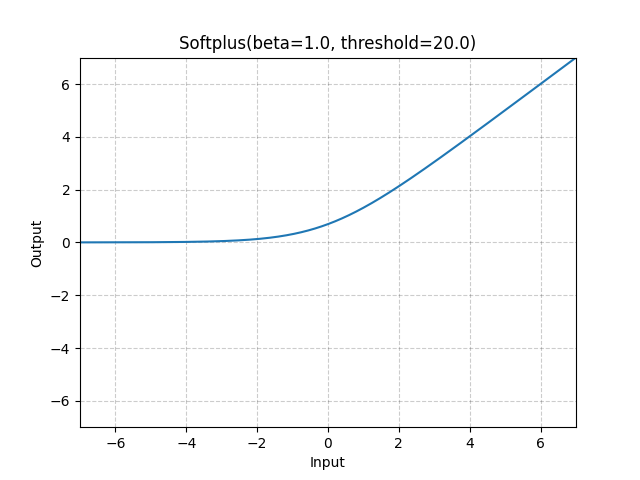
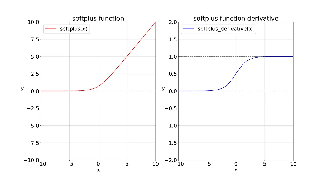
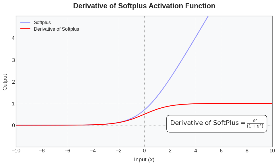
This is the graph for the Softplus function and its derivative.

# !/usr/bin/env python
# coding=utf-8

import torch
from matplotlib import pyplot as plt


def plot(X, Y=None, xlabel=None, ylabel=None, legend=[], xlim=None, ylim=None, xscale='linear', yscale='linear',
         fmts=('-', 'm--', 'g-.', 'r:'), figsize=(3.5, 2.5), axes=None):
    """
    https://github.com/d2l-ai/d2l-en/blob/master/d2l/torch.py
    """

    def has_one_axis(X):  # True if X (tensor or list) has 1 axis
        return ((hasattr(X, "ndim") and (X.ndim == 1)) or (isinstance(X, list) and (not hasattr(X[0], "__len__"))))

    if has_one_axis(X): X = [X]

    if Y is None:
        X, Y = [[]] * len(X), X
    elif has_one_axis(Y):
        Y = [Y]

    if len(X) != len(Y):
        X = X * len(Y)

    # Set the default width and height of figures globally, in inches.
    plt.rcParams['figure.figsize'] = figsize

    if axes is None:
        axes = plt.gca()  # Get the current Axes

    # Clear the Axes
    axes.cla()

    for x, y, fmt in zip(X, Y, fmts):
        axes.plot(x, y, fmt) if len(x) else axes.plot(y, fmt)

    axes.set_xlabel(xlabel), axes.set_ylabel(ylabel)  # Set the label for the x/y-axis
    axes.set_xscale(xscale), axes.set_yscale(yscale)  # Set the x/y-axis scale
    axes.set_xlim(xlim), axes.set_ylim(ylim)  # Set the x/y-axis view limits

    if legend:
        axes.legend(legend)  # Place a legend on the Axes

    # Configure the grid lines
    axes.grid()

    plt.show()
    plt.savefig("yongqiang.png", transparent=True)  # Save the current figure


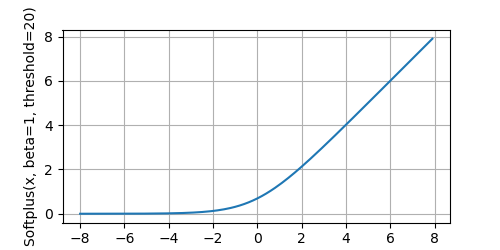
x = torch.arange(-8.0, 8.0, 0.1, requires_grad=True)
y = torch.nn.functional.softplus(x, beta=1, threshold=20)
plot(x.detach(), y.detach(), 'x', 'Softplus(x, beta=1, threshold=20)', figsize=(5, 2.5))

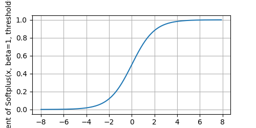
# Clear out previous gradients
# x.grad.data.zero_()
y.backward(torch.ones_like(x), retain_graph=True)
plot(x.detach(), x.grad, 'x', 'gradient of Softplus(x, beta=1, threshold=20)', figsize=(5, 2.5))

The Softplus function:

The derivative of the Softplus function:

Softplus function is a smooth approximation of the ReLU function.

1. Smooth Approximation of ReLU: The Softplus function is often seen as a smoother version of the ReLU function. While ReLU is simple and effective, it can have issues, such as causing neurons to "die" if they always output zero for negative inputs. Softplus avoids this issue by providing a smooth, continuous output for both positive and negative inputs.

2. Differentiability: Softplus is a differentiable function, unlike ReLU, which has a discontinuity at zero. The continuous and differentiable nature of Softplus makes it easier for gradient-based optimization algorithms to work effectively, ensuring smooth learning during training.

3. Preventing Dying Neurons: In the case of ReLU, when the input is negative, the output is exactly zero, which can lead to dead neurons that do not contribute to learning. Softplus gradually approaches zero for negative values, ensuring that neurons always produce some non-zero output and continue contributing to the learning process.

4. Numerical Stability: The Softplus function has better numerical stability than some other activation functions because it avoids the issues that arise from very large or very small values. It has a smooth output, and for very large or very small inputs, the function behaves predictably, reducing the risk of overflow or underflow in computations.

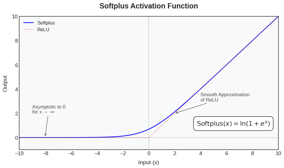
The Softplus function outputs values from 0 to infinity. This ensures that it can be used in situations where positive outputs are desired, such as in regression tasks where the outputs should be non-negative.

As x → ∞ x \rightarrow \infty x→∞, Softplus behaves like a linear function:

∑ x → ∞ = ln ( 1 + e x ) ≈ x \begin{aligned} \sum_{x \rightarrow \infty}^{} = \text{ln}(1 + e^{x}) \approx x \\ \end{aligned} x→∞∑=ln(1+ex)≈x

As x → − ∞ x \rightarrow -\infty x→−∞, Softplus approaches zero, but never actually reaches zero. This helps to avoid the problem of dead neurons, which is common in ReLU when the input is negative:

∑ x → − ∞ = ln ( 1 + e x ) ≈ 0 \begin{aligned} \sum_{x \rightarrow -\infty}^{} = \text{ln}(1 + e^{x}) \approx 0 \\ \end{aligned} x→−∞∑=ln(1+ex)≈0

2. Softplus Function - Derivatives and Gradients (导数和梯度)

Notes

• Element-wise Multiplication (Hadamard Product) (* operator or numpy.multiply()): Multiplies corresponding elements of two arrays that must have the same shape (or be broadcastable to a common shape).
• Matrix Multiplication (Dot Product) (@ operator or numpy.matmul() or numpy.dot()): Performs the standard linear algebra operation that requires specific dimension compatibility rules. (e.g., the number of columns in the first array must match the number of rows in the second).

2.1. PyTorch torch.nn.Softplus(beta=1.0, threshold=20.0)

# !/usr/bin/env python
# coding=utf-8

import torch
import torch.nn as nn

torch.set_printoptions(precision=6)

input = torch.tensor([[-1.5, 0.0, 1.5], [0.5, -2.0, 3.0]], dtype=torch.float, requires_grad=True)

print(f"input.requires_grad: {input.requires_grad}, input.shape: {input.shape}")

forward_output = torch.nn.functional.softplus(input, beta=1, threshold=20)
print(f"\nforward_output.shape: {forward_output.shape}")
print(f"Forward Pass Output:\n{forward_output}")

forward_output.backward(torch.ones_like(input), retain_graph=True)

print(f"\nbackward_output.shape: {input.grad.shape}")
print(f"Backward Pass Output:\n{input.grad}")

/home/yongqiang/miniconda3/bin/python /home/yongqiang/quantitative_analysis/softplus.py 
input.requires_grad: True, input.shape: torch.Size([2, 3])

forward_output.shape: torch.Size([2, 3])
Forward Pass Output:
tensor([[0.201413, 0.693147, 1.701413],
        [0.974077, 0.126928, 3.048587]], grad_fn=<SoftplusBackward0>)

backward_output.shape: torch.Size([2, 3])
Backward Pass Output:
tensor([[0.182426, 0.500000, 0.817575],
        [0.622459, 0.119203, 0.952574]])

Process finished with exit code 0

2.2. PyTorch torch.nn.Softplus(beta=1.0, threshold=20.0)

# !/usr/bin/env python
# coding=utf-8

import torch
import torch.nn as nn

torch.set_printoptions(precision=6)

input = torch.tensor([-1.5, 0.0, 1.5, 0.5, -2.0, 3.0], dtype=torch.float, requires_grad=True)

print(f"input.requires_grad: {input.requires_grad}, input.shape: {input.shape}")

forward_output = torch.nn.functional.softplus(input, beta=1, threshold=20)
print(f"\nforward_output.shape: {forward_output.shape}")
print(f"Forward Pass Output:\n{forward_output}")

forward_output.backward(torch.ones_like(input), retain_graph=True)

print(f"\nbackward_output.shape: {input.grad.shape}")
print(f"Backward Pass Output:\n{input.grad}")

/home/yongqiang/miniconda3/bin/python /home/yongqiang/quantitative_analysis/softplus.py 
input.requires_grad: True, input.shape: torch.Size([6])

forward_output.shape: torch.Size([6])
Forward Pass Output:
tensor([0.201413, 0.693147, 1.701413, 0.974077, 0.126928, 3.048587],
       grad_fn=<SoftplusBackward0>)

backward_output.shape: torch.Size([6])
Backward Pass Output:
tensor([0.182426, 0.500000, 0.817575, 0.622459, 0.119203, 0.952574])

Process finished with exit code 0

2.3. Python Softplus Function

# !/usr/bin/env python
# coding=utf-8

import numpy as np


# numpy.multiply:
# Multiply arguments element-wise
# Equivalent to x1 * x2 in terms of array broadcasting

class SoftplusLayer:
    """
    A class to represent the Softplus layer for a neural network.
    """

    def __init__(self, beta=1.0, threshold=20.0):
        self.beta = beta
        self.threshold = threshold
        # Cache the input for the backward pass
        self.input = None

    def forward(self, input):
        """
        Forward Pass: f(x) = 1/beta * log(1 + exp(beta * x))
        Uses linear approximation f(x) = ln(1 + exp(x)) = x for (beta * x) > threshold to prevent overflow
        """

        self.input = input
        val = self.beta * input
        output = np.where(val > self.threshold, input, (1.0 / self.beta) * np.log(1 + np.exp(val)))
        return output

    def backward(self, upstream_gradient):
        """
        Backward Pass (Backpropagation): f'(x) = 1 / (1 + exp(-beta * x))
        The total gradient is the element-wise product of the upstream
        gradient and the derivative of the Softplus.
        """

        val = self.beta * self.input
        sigmoid = 1.0 / (1.0 + np.exp(-val))
        print(f"softplus_derivative.shape: {sigmoid.shape}")
        print(f"Softplus Derivative:\n{sigmoid}")

        # Computes the gradient of the loss with respect to the input (dL/dx)
        # Apply the chain rule: multiply the derivative by the upstream gradient
        # dL/dx = dL/dy * dy/dx = upstream_gradient * f'(x)
        downstream_gradient = upstream_gradient * sigmoid
        return downstream_gradient


layer = SoftplusLayer()

input = np.array([-1.5, 0.0, 1.5, 0.5, -2.0, 3.0], dtype=np.float32)

# Forward pass
forward_output = layer.forward(input)
print(f"\nforward_output.shape: {forward_output.shape}")
print(f"Forward Pass Output:\n{forward_output}")

# Backward pass
upstream_gradient = np.ones(forward_output.shape) * 0.1
backward_output = layer.backward(upstream_gradient)
print(f"\nbackward_output.shape: {backward_output.shape}")
print(f"Backward Pass Output:\n{backward_output}")

/home/yongqiang/miniconda3/bin/python /home/yongqiang/quantitative_analysis/softplus.py 

forward_output.shape: (6,)
Forward Pass Output:
[0.20141323 0.6931472  1.7014133  0.974077   0.12692805 3.0485873 ]
softplus_derivative.shape: (6,)
Softplus Derivative:
[0.18242553 0.5        0.8175745  0.62245935 0.11920293 0.95257413]

backward_output.shape: (6,)
Backward Pass Output:
[0.01824255 0.05       0.08175745 0.06224594 0.01192029 0.09525741]

Process finished with exit code 0

2.4. Python Softplus Function

# !/usr/bin/env python
# coding=utf-8

import numpy as np


# numpy.multiply:
# Multiply arguments element-wise
# Equivalent to x1 * x2 in terms of array broadcasting

class SoftplusLayer:
    """
    A class to represent the Softplus layer for a neural network.
    """

    def __init__(self, beta=1.0, threshold=20.0):
        self.beta = beta
        self.threshold = threshold
        # Cache the input for the backward pass
        self.input = None

    def forward(self, input):
        """
        Forward Pass: f(x) = 1/beta * log(1 + exp(beta * x))
        Uses linear approximation f(x) = ln(1 + exp(x)) = x for (beta * x) > threshold to prevent overflow
        """

        self.input = input
        val = self.beta * input
        output = np.where(val > self.threshold, input, (1.0 / self.beta) * np.log(1 + np.exp(val)))
        return output

    def backward(self, upstream_gradient):
        """
        Backward Pass (Backpropagation): f'(x) = 1 / (1 + exp(-beta * x))
        The total gradient is the element-wise product of the upstream
        gradient and the derivative of the Softplus.
        """

        val = self.beta * self.input
        sigmoid = 1.0 / (1.0 + np.exp(-val))
        print(f"softplus_derivative.shape: {sigmoid.shape}")
        print(f"Softplus Derivative:\n{sigmoid}")

        # Computes the gradient of the loss with respect to the input (dL/dx)
        # Apply the chain rule: multiply the derivative by the upstream gradient
        # dL/dx = dL/dy * dy/dx = upstream_gradient * f'(x)
        downstream_gradient = upstream_gradient * sigmoid
        return downstream_gradient


layer = SoftplusLayer()

input = np.array([[-1.5, 0.0, 1.5], [0.5, -2.0, 3.0]], dtype=np.float32)

# Forward pass
forward_output = layer.forward(input)
print(f"\nforward_output.shape: {forward_output.shape}")
print(f"Forward Pass Output:\n{forward_output}")

# Backward pass
upstream_gradient = np.ones(forward_output.shape) * 0.1
backward_output = layer.backward(upstream_gradient)
print(f"\nbackward_output.shape: {backward_output.shape}")
print(f"Backward Pass Output:\n{backward_output}")

/home/yongqiang/miniconda3/bin/python /home/yongqiang/quantitative_analysis/softplus.py 

forward_output.shape: (2, 3)
Forward Pass Output:
[[0.20141323 0.6931472  1.7014133 ]
 [0.974077   0.12692805 3.0485873 ]]
softplus_derivative.shape: (2, 3)
Softplus Derivative:
[[0.18242553 0.5        0.8175745 ]
 [0.62245935 0.11920293 0.95257413]]

backward_output.shape: (2, 3)
Backward Pass Output:
[[0.01824255 0.05       0.08175745]
 [0.06224594 0.01192029 0.09525741]]

Process finished with exit code 0

References

1\] Yongqiang Cheng (程永强), \[2\] 动手学深度学习, \[3\] Deep Learning Tutorials, \[4\] Gradient boosting performs gradient descent, \[5\] Matrix calculus, \[6\] Artificial Inteligence, \[7\] Softplus Function in Neural Network,