【微科普】BERT 主题建模 + 多模态分析，解锁阆中古镇评论数据价值

目录

一、核心原理速懂

[1. BERT 主题建模：比传统方法更懂中文评论](#1. BERT 主题建模：比传统方法更懂中文评论)

[2. 多模态分析：不止于文字，多维挖掘数据价值](#2. 多模态分析：不止于文字，多维挖掘数据价值)

[二、Python 代码实战：从数据加载到主题可视化](#二、Python 代码实战：从数据加载到主题可视化)

第一步：安装依赖库

第二步：完整代码（含注释）

三、结果解读指南

四、小贴士

一、核心原理速懂

1. BERT 主题建模：比传统方法更懂中文评论

传统主题模型（如 LDA）靠统计词频找主题，容易忽略语境（比如 "古城夜景" 和 "夜景一般" 的 "夜景" 语义差异）。而 BERT 作为预训练语言模型，能深度理解中文语义：

• 先将评论文本转化为计算机能识别的 "语义向量"（捕捉词语上下文关系）；
• 再通过聚类算法（如 K-Means）将语义相似的向量归为一类，每类就是一个核心主题；
• 最后从每类中提取高频关键词，就能清晰看到游客关注的核心话题（比如 "古建筑""美食""交通"）。

2. 多模态分析：不止于文字，多维挖掘数据价值

前阵子获取的大众点评数据包含 "用户名、时间、情感、评分、评论" 等 8 列，这就是天然的多模态数据：

• 文本模态：评论内容（分词后、去停用词）→ 用 BERT 挖主题；
• 数值模态：评分→ ；
• 分类模态：情感（正面 / 负面）→ 看不同主题的情感倾向（比如 "交通" 主题是否负面评论多）；
• 时间模态：评论时间→ 分析主题随时间变化（比如节假日游客更关注 "拥挤度"）。

二、Python 代码实战：从数据加载到主题可视化

第一步：安装依赖库

# 核心库：BERT向量生成、主题聚类、数据处理、可视化
pip install torch transformers scikit-learn pandas numpy matplotlib seaborn openpyxl

第二步：完整代码（含注释）

import pandas as pd
import numpy as np
import matplotlib.pyplot as plt
from sklearn.cluster import KMeans
from sklearn.metrics import silhouette_score
from transformers import BertTokenizer, BertModel
import torch
import seaborn as sns
from collections import Counter

# ----------------------1. 数据加载与预处理----------------------
# 读取Excel数据（A-H列自动识别）
df = pd.read_excel("景区评论数据_分词后.xlsx", engine="openpyxl")

# 筛选有效数据（仅保留有"分词结果_去停用词"和"评分""情感"的行）
df = df.dropna(subset=["分词结果_去停用词", "评分", "情感", "时间"])
df.reset_index(drop=True, inplace=True)

# 准备文本数据（将分词结果拼接成完整句子，适配BERT输入）
df["text_for_bert"] = df["分词结果_去停用词"].apply(lambda x: " ".join(eval(x)) if isinstance(x, str) else "")

# ----------------------2. BERT生成语义向量----------------------
# 加载中文BERT模型（轻量版，速度快，适合小数据）
tokenizer = BertTokenizer.from_pretrained("bert-base-chinese")
model = BertModel.from_pretrained("bert-base-chinese")

# 定义向量生成函数（批量处理，避免内存溢出）
def get_bert_embeddings(texts, batch_size=32):
    embeddings = []
    for i in range(0, len(texts), batch_size):
        batch_texts = texts[i:i+batch_size]
        # BERT输入编码（max_length=50：评论长度限制为50词，按需调整）
        inputs = tokenizer(
            batch_texts,
            padding=True,
            truncation=True,
            max_length=50,
            return_tensors="pt"
        )
        # 生成向量（取[CLS] token的输出作为句子语义向量）
        with torch.no_grad():
            outputs = model(**inputs)
            batch_embeds = outputs.last_hidden_state[:, 0, :].numpy()
        embeddings.extend(batch_embeds)
    return np.array(embeddings)

# 生成所有评论的BERT向量
print("正在生成BERT语义向量...")
texts = df["text_for_bert"].tolist()
bert_vectors = get_bert_embeddings(texts)

# ----------------------3. K-Means聚类找主题（自动选最优聚类数）----------------------
# 计算不同聚类数的轮廓系数（越大聚类效果越好）
silhouette_scores = []
k_range = range(2, 8)  # 假设主题数在2-7之间
for k in k_range:
    kmeans = KMeans(n_clusters=k, random_state=42)
    cluster_labels = kmeans.fit_predict(bert_vectors)
    silhouette_scores.append(silhouette_score(bert_vectors, cluster_labels))

# 可视化轮廓系数，选最优k
plt.figure(figsize=(8, 4))
plt.plot(k_range, silhouette_scores, marker="o")
plt.xlabel("主题数量k")
plt.ylabel("轮廓系数")
plt.title("阆中古镇评论-最优主题数选择")
plt.savefig("最优主题数.png", dpi=300, bbox_inches="tight")
plt.show()

# 最优k值（取轮廓系数最大的k）
best_k = k_range[silhouette_scores.index(max(silhouette_scores))]
print(f"最优主题数：{best_k}")

# 最终聚类
kmeans = KMeans(n_clusters=best_k, random_state=42)
df["主题标签"] = kmeans.fit_predict(bert_vectors)

# ----------------------4. 提取主题关键词（每类Top10关键词）----------------------
def get_topic_keywords(df, topic_id, top_n=10):
    # 筛选该主题的所有评论分词结果
    topic_texts = df[df["主题标签"] == topic_id]["分词结果_去停用词"]
    # 统计所有词的频率
    word_counts = Counter()
    for text in topic_texts:
        word_counts.update(eval(text) if isinstance(text, str) else [])
    # 返回Top10高频词
    return word_counts.most_common(top_n)

# 输出所有主题的关键词
topics_keywords = {}
for i in range(best_k):
    keywords = get_topic_keywords(df, i)
    topics_keywords[f"主题{i+1}"] = [word for word, count in keywords]
    print(f"\n主题{i+1}关键词：{topics_keywords[f'主题{i+1}']}")

# ----------------------5. 多模态分析（主题+情感+评分+时间）----------------------
# 5.1 主题与情感分布（看每个主题的正负情感占比）
topic_emotion = pd.crosstab(df["主题标签"], df["情感"], normalize="index") * 100
print("\n主题-情感分布（%）：")
print(topic_emotion)

# 可视化：堆叠柱状图
plt.figure(figsize=(10, 6))
topic_emotion.plot(kind="bar", stacked=True, colormap="RdYlGn")
plt.xlabel("主题标签")
plt.ylabel("情感占比（%）")
plt.title("阆中古镇各主题情感分布")
plt.xticks(ticks=range(best_k), labels=[f"主题{i+1}" for i in range(best_k)], rotation=0)
plt.legend(title="情感")
plt.savefig("主题-情感分布.png", dpi=300, bbox_inches="tight")
plt.show()

# 5.2 主题与评分关联（看每个主题的平均评分）
topic_rating = df.groupby("主题标签")["评分"].agg(["mean", "count"]).round(2)
topic_rating.columns = ["平均评分", "评论数量"]
print("\n主题-评分统计：")
print(topic_rating)

# 可视化：柱状图
plt.figure(figsize=(10, 6))
sns.barplot(x=topic_rating.index, y="平均评分", data=topic_rating, palette="Blues")
plt.xlabel("主题标签")
plt.ylabel("平均评分")
plt.title("阆中古镇各主题平均评分")
plt.xticks(ticks=range(best_k), labels=[f"主题{i+1}" for i in range(best_k)], rotation=0)
# 在柱子上标注评论数量
for i, count in enumerate(topic_rating["评论数量"]):
    plt.text(i, topic_rating["平均评分"][i] + 0.1, f"n={count}", ha="center")
plt.savefig("主题-平均评分.png", dpi=300, bbox_inches="tight")
plt.show()

# 5.3 主题随时间变化（按月份统计各主题评论数）
# 时间格式转换（假设时间列是字符串，转为datetime）
df["时间"] = pd.to_datetime(df["时间"], errors="coerce")
df["月份"] = df["时间"].dt.to_period("M")  # 按月份分组

# 统计每月各主题评论数
topic_time = pd.crosstab(df["月份"], df["主题标签"])
print("\n主题-时间分布：")
print(topic_time)

# 可视化：折线图
plt.figure(figsize=(12, 6))
topic_time.plot(kind="line", marker="o")
plt.xlabel("时间（月份）")
plt.ylabel("评论数量")
plt.title("阆中古镇各主题随时间变化趋势")
plt.legend(title="主题标签", labels=[f"主题{i+1}" for i in range(best_k)])
plt.xticks(rotation=45)
plt.tight_layout()
plt.savefig("主题-时间趋势.png", dpi=300, bbox_inches="tight")
plt.show()

# ----------------------6. 结果保存（便于后续分析）----------------------
# 给主题标签添加关键词备注
df["主题名称"] = df["主题标签"].apply(lambda x: f"主题{x+1}：{'-'.join(topics_keywords[f'主题{x+1}'][:3])}")
# 保存到新Excel
df.to_excel("阆中古镇评论_主题分析结果.xlsx", index=False, engine="openpyxl")
print("\n分析结果已保存到：阆中古镇评论_主题分析结果.xlsx")

三、结果解读指南

1. 主题识别：看 "主题关键词"，比如主题 1 关键词是 "古建筑 - 张飞庙 - 中天楼"，说明这是 "历史景点打卡" 主题；主题 2 是 "醋 - 张飞牛肉 - 美食"，就是 "当地美食体验" 主题。
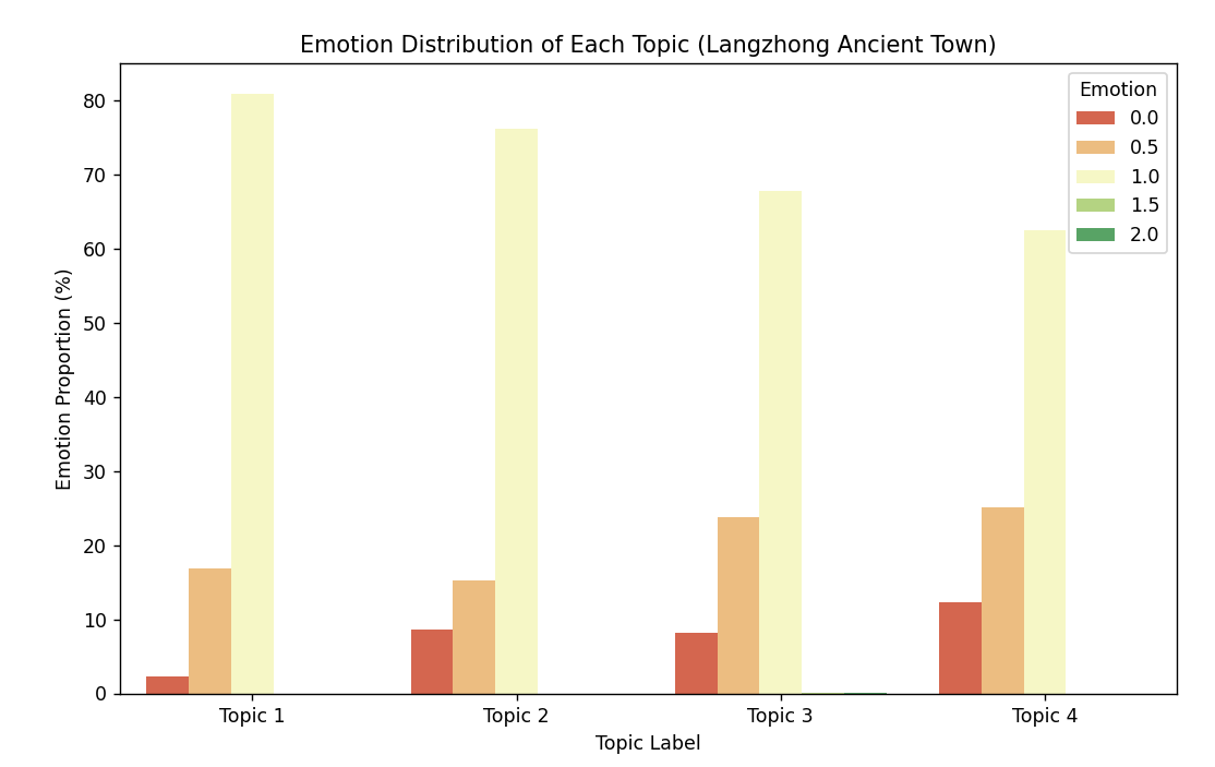
2. 情感倾向：如果 "交通" 主题负面情感占比高，说明游客对交通便利性满意度低；
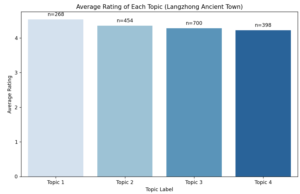
3. 评分关联：如果 "美食" 主题平均评分 4.8 分（满分 5 分），说明美食是核心优势；
4. 时间趋势：如果节假日 "拥挤 - 排队" 主题评论增多，说明景区需要优化客流管控。

四、小贴士

• 若评论数据量较大（万级以上），可换 "bert-base-chinese-finetuned-sentiment" 微调模型，速度更快；
• 停用词可自定义（比如添加 "阆中""古镇" 等无意义高频词），让关键词更精准；
• 多模态还能拓展：比如结合用户画像（用户名是否重复）分析回头客关注的主题。

附------调试日志

'(MaxRetryError("HTTPSConnectionPool(host='huggingface.co', port=443): Max retries exceeded with url: /bert-base-chinese/resolve/main/vocab.txt (Caused by ConnectTimeoutError(<HTTPSConnection(host='huggingface.co', port=443) at 0x26b0ca029a0>, 'Connection to huggingface.co timed out. (connect timeout=10)'))"), '(Request ID: 39283957-dc99-419f-a54b-f6196b397ed2)')' thrown while requesting HEAD https://huggingface.co/bert-base-chinese/resolve/main/vocab.txt Retrying in 1s [Retry 1/5].

无法连接到 HuggingFace 服务器下载 BERT 模型 （网络超时），解决方法是手动下载 BERT 模型到本地，再加载，步骤如下：

步骤 1：手动下载bert-base-chinese模型文件

打开浏览器，访问bert-base-chinese的 HuggingFace 仓库：https://huggingface.co/bert-base-chinese/tree/main

（这个网址也打不开，开了梯子才行）

下载以下 5 个核心文件到本地文件夹（比如命名为bert-base-chinese-local）：

• config.json
• pytorch_model.bin
• tokenizer_config.json
• vocab.txt
• special_tokens_map.json

步骤 2：修改代码，从本地加载模型

把原来加载tokenizer和model的代码，替换为本地路径加载：

# 原来的代码（注释掉）
# tokenizer = BertTokenizer.from_pretrained("bert-base-chinese")
# model = BertModel.from_pretrained("bert-base-chinese")

# 新代码：从本地文件夹加载
tokenizer = BertTokenizer.from_pretrained("./bert-base-chinese-local")  # 本地文件夹路径
model = BertModel.from_pretrained("./bert-base-chinese-local")

额外说明

• 如果是国内网络，也可以通过国内镜像源加速下载（但手动下载更稳定）；
• 确保本地文件夹路径正确（比如代码和bert-base-chinese-local文件夹在同一目录下）。

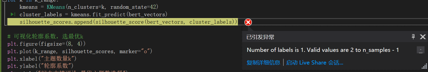
这个报错的原因是轮廓系数（silhouette_score）的计算要求聚类数至少为 2，但当前代码中某一次聚类后只得到了 1 个类别。

问题分析

轮廓系数的计算逻辑是 "衡量样本与自身聚类的相似度，以及与其他聚类的差异"，因此必须至少有 2 个聚类类别才能计算。出现该错误通常是因为：

1. 数据量过少（比如有效评论数不足 10 条），K-Means 无法分成多个类别；
2. 聚类数k的取值不合理（比如k大于样本数）；
3. 文本语义过于单一，所有评论的 BERT 向量都高度相似，聚类后只能得到 1 类。

数据中存在大量重复的 BERT 向量（即多条评论的语义完全一致），导致 K-Means 聚类时无法分成 2 个类别，最终只得到 1 个簇。

分词结果_去停用词列的内容是 "空格分隔的字符串"，不是 "列表格式的字符串" ，所以ast.literal_eval解析失败，导致text_for_bert全为空。

解决方法：直接按空格拆分分词结果（不需要ast.literal_eval），修改parse_segmented_text函数

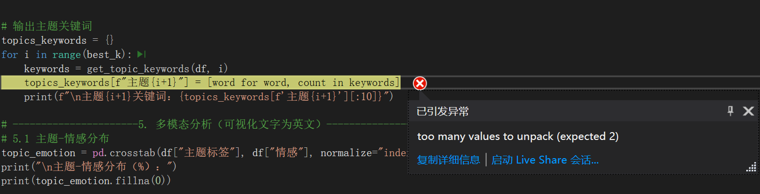
这个报错 "too many values to unpack (expected 2)" 的原因是：get_topic_keywords函数返回的结果格式不符合预期（需要返回 "(词，词频)" 的二元组，但实际返回的是单个元素）。

问题分析

你之前可能修改了get_topic_keywords函数（比如改用了 TF-IDF 方案），导致它返回的是单个词的列表 ，而非原来的 "(词，词频)" 二元组列表，因此在[word for word, count in keywords]这一步无法拆包。

代码运行结果：

输出：

解析后的text_for_bert内容（前5条）：

0 值得 一去 古色古香 不愧 5 级 景区 靠近 江边 木质 建筑 朴实 真的 很大 感觉 逛...

1 听说 春节 发源地 很大 一天 可能 逛 完会 一点 说实话 景区 里面 打造 有点 失败 ...

2 不妨 来到 时间 放慢 些 三月份 汉服 文化节 宜宾 赶过去 看 几个 朋友 一起 拍照 ...

3 适合 慢下来 真的 好大 古老 墙 小院 开发 挺 好 道路 适合 行人 管理 不错 唯一 ...

4 感觉 古镇 差不多 专门 开 2 小时 车 感觉 集市 买 牛肉 味道 不错

Name: text_for_bert, dtype: object

正在生成BERT语义向量...

原始向量数：1820，去重后向量数：1820

手动指定主题数：3

主题1关键词：['张飞', '牛肉', '地方', '嘉陵江', '四大', '春节', '历史', '古镇', '感觉', '真的']

主题2关键词：['古镇', '里面', '牛肉', '不错', '景点', '感觉', '地方', '比较', '没有', '张飞']

主题3关键词：['牛肉', '张飞', '景点', '保宁', '嘉陵江', '特色', '四大', '中国', '历史', '不错']

主题-情感分布（%）：

情感 0.0 0.5 1.0 1.5 2.0

主题标签

0 8.884298 15.495868 75.619835 0.000000 0.000000

1 7.989348 23.435419 68.308921 0.133156 0.133156

2 8.205128 22.051282 69.743590 0.000000 0.000000

主题-评分统计：

平均评分 评论数量

主题标签

0 4.35 484

1 4.29 751

2 4.34 585

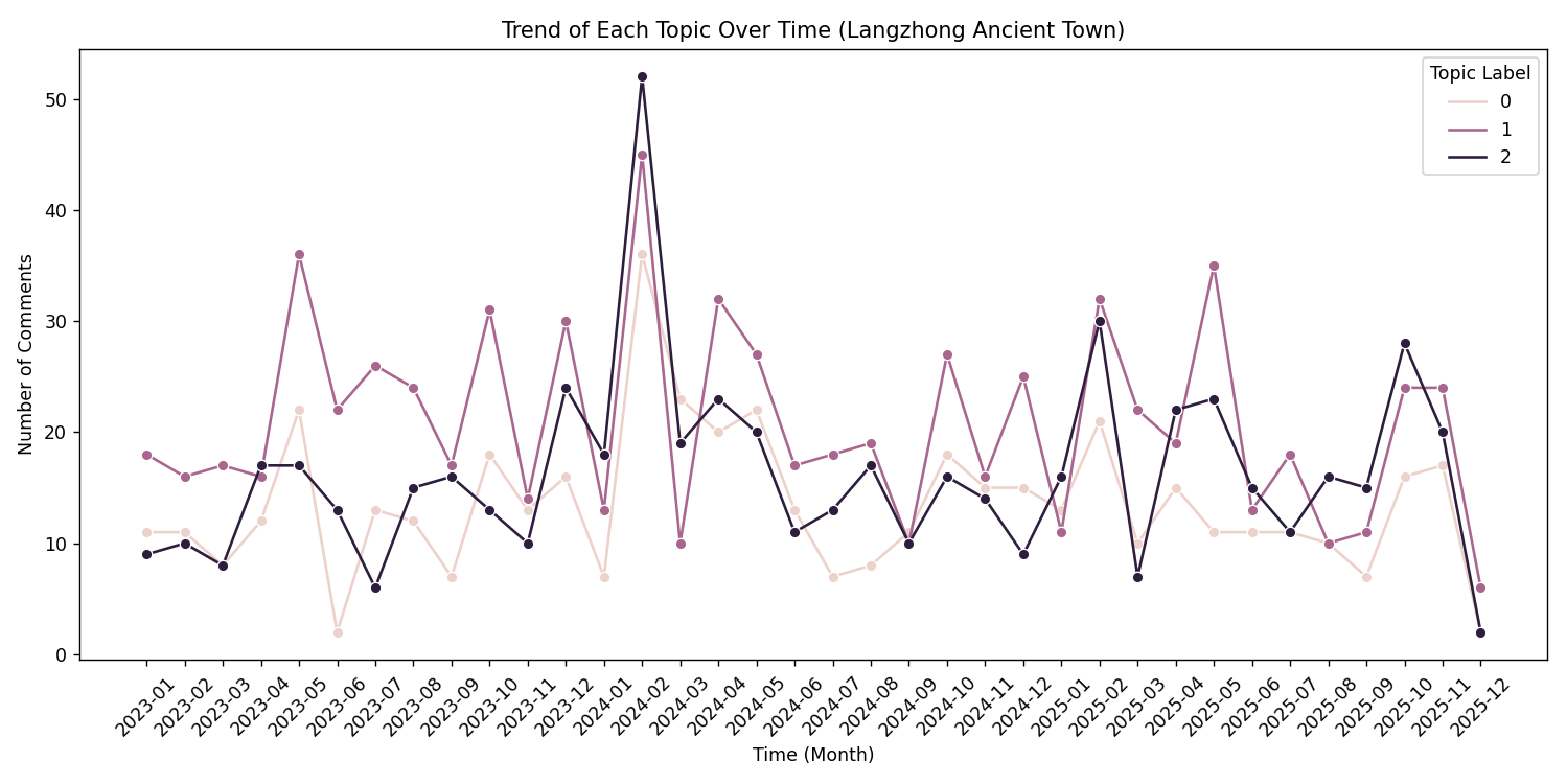
主题-时间分布：

主题标签 0 1 2

月份

2023-01 11 18 9

2023-02 11 16 10

2023-03 8 17 8

2023-04 12 16 17

2023-05 22 36 17

2023-06 2 22 13

2023-07 13 26 6

2023-08 12 24 15

2023-09 7 17 16

2023-10 18 31 13

2023-11 13 14 10

2023-12 16 30 24

2024-01 7 13 18

2024-02 36 45 52

2024-03 23 10 19

2024-04 20 32 23

2024-05 22 27 20

2024-06 13 17 11

2024-07 7 18 13

2024-08 8 19 17

2024-09 11 10 10

2024-10 18 27 16

2024-11 15 16 14

2024-12 15 25 9

2025-01 13 11 16

2025-02 21 32 30

2025-03 10 22 7

2025-04 15 19 22

2025-05 11 35 23

2025-06 11 13 15

2025-07 11 18 11

2025-08 10 10 16

2025-09 7 11 15

2025-10 16 24 28

2025-11 17 24 20

2025-12 2 6 2

import pandas as pd
import numpy as np
import matplotlib.pyplot as plt
from sklearn.cluster import KMeans
from sklearn.metrics import silhouette_score
from sklearn.preprocessing import StandardScaler
from sklearn.feature_extraction.text import TfidfVectorizer
from transformers import BertTokenizer, BertModel
import torch
import seaborn as sns
from collections import Counter

# ----------------------1. 数据加载与预处理（含停用词过滤）----------------------
# 读取Excel数据
df = pd.read_excel("景区评论数据_分词后.xlsx", engine="openpyxl")

# 筛选有效数据
df = df.dropna(subset=["分词结果_去停用词", "评分", "情感", "时间"])
df.reset_index(drop=True, inplace=True)

# 定义需要去除的停用词
stopwords = {"古城", "很", "都", "阆中", "去", "人", "很多", "还", "不"}

# 解析分词结果并过滤停用词
def parse_and_remove_stopwords(x):
    if not isinstance(x, str):
        return ""
    words = x.strip().split()
    filtered_words = [word for word in words if word not in stopwords]
    return " ".join(filtered_words) if len(filtered_words) > 0 else ""

df["text_for_bert"] = df["分词结果_去停用词"].apply(parse_and_remove_stopwords)

# 过滤空文本
df = df[df["text_for_bert"] != ""].reset_index(drop=True)
if len(df) == 0:
    raise ValueError("无有效评论文本，请检查分词结果列格式")

# 打印解析后的结果（验证）
print("解析后的text_for_bert内容（前5条）：")
print(df["text_for_bert"].head(5))

# ----------------------2. BERT生成语义向量----------------------
# 加载本地BERT模型
tokenizer = BertTokenizer.from_pretrained("./bert-base-chinese-local")
model = BertModel.from_pretrained("./bert-base-chinese-local")
model.eval()  # 设为评估模式

# 批量生成BERT语义向量
def get_bert_embeddings(texts, batch_size=32):
    embeddings = []
    for i in range(0, len(texts), batch_size):
        batch_texts = texts[i:i+batch_size]
        inputs = tokenizer(
            batch_texts,
            padding=True,
            truncation=True,
            max_length=50,
            return_tensors="pt"
        )
        with torch.no_grad():
            outputs = model(**inputs)
            # 取[CLS]位置的向量作为句子表示
            batch_embeds = outputs.last_hidden_state[:, 0, :].numpy()
        embeddings.extend(batch_embeds)
    return np.array(embeddings)

print("\n正在生成BERT语义向量...")
texts = df["text_for_bert"].tolist()
bert_vectors = get_bert_embeddings(texts)

# 向量标准化（提升聚类稳定性）
scaler = StandardScaler()
bert_vectors_scaled = scaler.fit_transform(bert_vectors)

# ----------------------3. K-Means聚类（手动指定主题数为4）----------------------
# 对向量去重
_, unique_indices = np.unique(bert_vectors_scaled, axis=0, return_index=True)
bert_vectors_unique = bert_vectors_scaled[np.sort(unique_indices)]
print(f"\n原始向量数：{len(bert_vectors_scaled)}，去重后向量数：{len(bert_vectors_unique)}")

# 手动指定主题数（避免分类过粗）
best_k = 3
print(f"手动指定主题数：{best_k}")

# 最终聚类并映射回原始数据
kmeans_final = KMeans(n_clusters=best_k, random_state=42, n_init=20)
unique_labels = kmeans_final.fit_predict(bert_vectors_unique)

vector_label_map = dict(zip(tuple(map(tuple, bert_vectors_unique)), unique_labels))
df["主题标签"] = [vector_label_map.get(tuple(vec), 0) for vec in bert_vectors_scaled]

# ----------------------4. 提取主题关键词（TF-IDF方案）----------------------
def get_topic_keywords(df, topic_id, top_n=10):
    # 提取该主题的所有评论（过滤停用词）
    topic_texts = df[df["主题标签"] == topic_id]["分词结果_去停用词"].apply(
        lambda x: " ".join([w for w in x.strip().split() if w not in stopwords])
    )
    # 过滤空文本
    topic_texts = topic_texts[topic_texts != ""]
    if len(topic_texts) == 0:
        return []
    # 用TF-IDF计算词权重（越低越能代表主题）
    tfidf = TfidfVectorizer()
    tfidf_matrix = tfidf.fit_transform(topic_texts)
    # 提取TopN关键词
    word_tfidf = dict(zip(tfidf.get_feature_names_out(), tfidf.idf_))
    sorted_words = sorted(word_tfidf.items(), key=lambda x: x[1], reverse=False)[:top_n]
    return [word for word, score in sorted_words]

# 输出主题关键词
topics_keywords = {}
for i in range(best_k):
    keywords = get_topic_keywords(df, i)
    topics_keywords[f"主题{i+1}"] = keywords
    print(f"\n主题{i+1}关键词：{topics_keywords[f'主题{i+1}'][:10]}")

# ----------------------5. 多模态分析（修复绘图渲染）----------------------
# 5.1 主题-情感分布
topic_emotion = pd.crosstab(df["主题标签"], df["情感"], normalize="index") * 100
print("\n主题-情感分布（%）：")
print(topic_emotion.fillna(0))

# 改用seaborn绘图（确保渲染）
plt.figure(figsize=(10, 6))
# 转换为长数据格式
topic_emotion_long = topic_emotion.reset_index().melt(
    id_vars="主题标签", var_name="Emotion", value_name="Proportion"
)
sns.barplot(
    x="主题标签", y="Proportion", hue="Emotion",
    data=topic_emotion_long, palette="RdYlGn"
)
plt.xlabel("Topic Label")
plt.ylabel("Emotion Proportion (%)")
plt.title("Emotion Distribution of Each Topic (Langzhong Ancient Town)")
plt.xticks(ticks=range(best_k), labels=[f"Topic {i+1}" for i in range(best_k)], rotation=0)
plt.legend(title="Emotion")
plt.savefig("主题-情感分布.png", dpi=300, bbox_inches="tight")
# 强制渲染
plt.draw()
plt.pause(0.5)
plt.show()

# 5.2 主题-评分统计
topic_rating = df.groupby("主题标签")["评分"].agg(["mean", "count"]).round(2)
topic_rating.columns = ["平均评分", "评论数量"]
print("\n主题-评分统计：")
print(topic_rating.fillna(0))

plt.figure(figsize=(10, 6))
sns.barplot(x=topic_rating.index, y="平均评分", data=topic_rating, palette="Blues")
plt.xlabel("Topic Label")
plt.ylabel("Average Rating")
plt.title("Average Rating of Each Topic (Langzhong Ancient Town)")
plt.xticks(ticks=range(best_k), labels=[f"Topic {i+1}" for i in range(best_k)], rotation=0)
for i, (mean_val, count) in enumerate(zip(topic_rating["平均评分"], topic_rating["评论数量"])):
    plt.text(i, mean_val + 0.1, f"n={count}", ha="center")
plt.savefig("主题-平均评分.png", dpi=300, bbox_inches="tight")
plt.draw()
plt.pause(0.5)
plt.show()
# 5.3 主题-时间趋势
df["时间"] = pd.to_datetime(df["时间"], errors="coerce")
df = df.dropna(subset=["时间"])
if len(df) >=1:
    # 将Period类型转为字符串
    df["月份"] = df["时间"].dt.to_period("M").astype(str)
    topic_time = pd.crosstab(df["月份"], df["主题标签"])
    print("\n主题-时间分布：")
    print(topic_time.fillna(0))

    plt.figure(figsize=(12, 6))
    # 转换为长数据格式
    topic_time_long = topic_time.reset_index().melt(
        id_vars="月份", var_name="Topic Label", value_name="Comment Count"
    )
    sns.lineplot(
        x="月份", y="Comment Count", hue="Topic Label",
        data=topic_time_long, marker="o"
    )
    plt.xlabel("Time (Month)")
    plt.ylabel("Number of Comments")
    plt.title("Trend of Each Topic Over Time (Langzhong Ancient Town)")
    plt.xticks(rotation=45)
    plt.tight_layout()
    plt.savefig("主题-时间趋势.png", dpi=300, bbox_inches="tight")
    plt.draw()
    plt.pause(0.5)
    plt.show()
else:
    print("无有效时间数据，跳过时间趋势分析")

# ----------------------6. 结果保存----------------------
df["主题名称"] = df["主题标签"].apply(lambda x: f"主题{x+1}：{'-'.join(topics_keywords[f'主题{x+1}'][:3])}")
df.to_excel("阆中古镇评论_主题分析结果.xlsx", index=False, engine="openpyxl")
print("\n分析结果已保存到：阆中古镇评论_主题分析结果.xlsx")