混合高斯模型全解析：原理，应用与代码实现

ming | 2026.01

如果你对混合高斯模型（GMM）还不太了解，不知道它能做什么，也完全没关系------本文正是为此而写。你只需要具备最基础的高斯分布（也称正态分布）知识即可轻松跟上。

这是一篇面向初学者的教程，本文将重点放在混合高斯分布的核心概念 与数学流程的梳理上，并会手把手带你用代码完成一个实际的应用示例。至于更深层的数学思想与模型设计方法技巧，本文暂不深入讨论，以帮助大家更快上手、理解该模型的核心用法。

本文中展示的示意图均为作者使用matplotlib原创绘制。读者可自由分享使用，但使用时请注明出处。

我们从最基础的高斯分布（也称正态分布）说起。以下这个概率密度函数想必大家再熟悉不过了，它不仅是概率论与统计中的核心分布，也是机器学习众多模型的基石：
<math xmlns="http://www.w3.org/1998/Math/MathML" display="block"> N ( x ∣ μ , σ ) = 1 2 π σ e − ( x − μ ) 2 2 σ 2 \mathcal{N}(x|\mu,\sigma) = \frac{1}{\sqrt{2\pi}\sigma} e^{\frac{-(x-\mu )^{2}}{2\sigma^{2}} } </math>N(x∣μ,σ)=2π σ1e2σ2−(x−μ)2

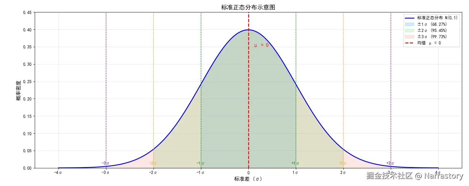
即使你之前已经学过，我们这里不妨一起回顾一下它的几个关键特性。该分布是关于 <math xmlns="http://www.w3.org/1998/Math/MathML"> x x </math>x的函数，并由两个参数决定：

<math xmlns="http://www.w3.org/1998/Math/MathML"> μ \mu </math>μ：均值，决定分布的中心位置，即对称轴所在；（读音为mu|缪）
<math xmlns="http://www.w3.org/1998/Math/MathML"> σ \sigma </math>σ：标准差，控制分布的离散程度；（读音为sigma | C个码）

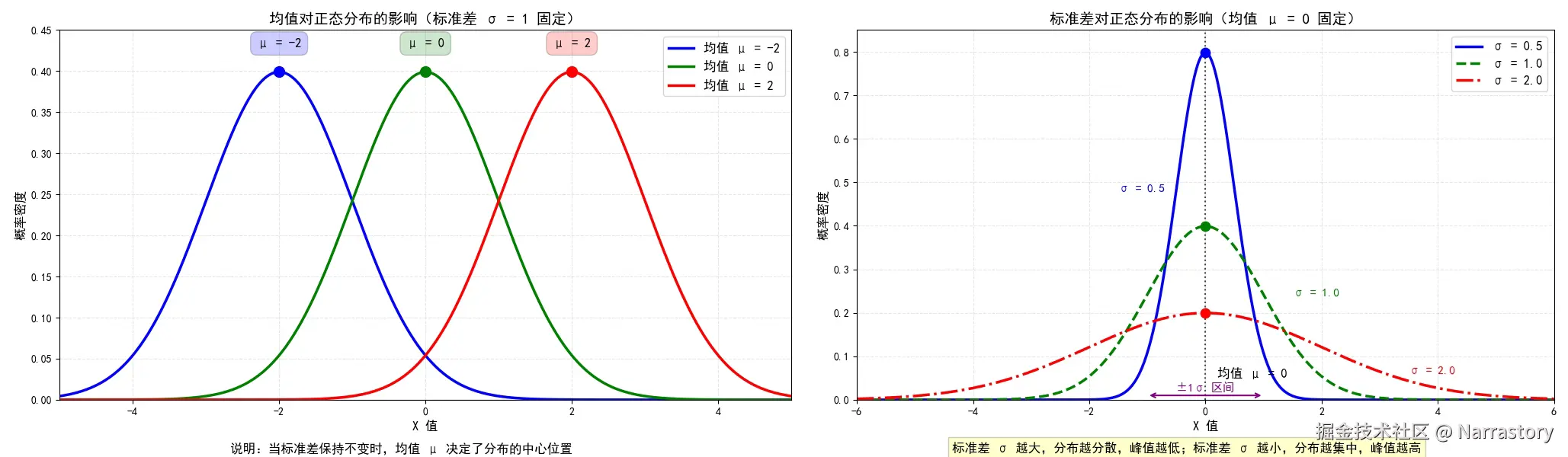
具体来说， <math xmlns="http://www.w3.org/1998/Math/MathML"> σ \sigma </math>σ 越大，曲线越"矮胖"，数据越分散； <math xmlns="http://www.w3.org/1998/Math/MathML"> σ \sigma </math>σ 越小，曲线越"高瘦"，数据越集中。下图直观展示了对不同 <math xmlns="http://www.w3.org/1998/Math/MathML"> μ \mu </math>μ 和 <math xmlns="http://www.w3.org/1998/Math/MathML"> σ \sigma </math>σ 时分布形态的变化：

用python实现这个高斯分布函数也非常简单，如下：

python 复制代码

import numpy as np
def gaussian_pdf_compact(x, mu, sigma):
    return np.exp(-0.5 * ((x - mu) / sigma) ** 2) / (sigma * np.sqrt(2 * np.pi))

现在，考虑下面这样的概率密度函数，你能否识别它属于哪种已知分布？或者，你能写出它的概率密度函数表达式 <math xmlns="http://www.w3.org/1998/Math/MathML"> f ( x ) f(x) </math>f(x)吗？

显然，这并不是我们常见的单一概率分布（如泊松分布、均匀分布等），而是一个形态复杂的非标准概率密度函数。然而，有趣的是，这个函数实际上是由三个不同的高斯分布（正态分布）经过加权叠加而成的。具体来说，它的数学表达式可以写为：
<math xmlns="http://www.w3.org/1998/Math/MathML" display="block"> f ( x ) = 1 3 × N ( x ∣ − 2.5 , 0.9 ) + 1 3 × N ( x ∣ 0.3 , 2 ) + 1 3 × N ( x ∣ 2.9 , 1.2 ) f(x) = \frac{1}{3} \times \mathcal{N}(x \mid -2.5,0.9) + \frac{1}{3} \times \mathcal{N}(x \mid0.3,2) + \frac{1}{3} \times \mathcal{N}(x \mid 2.9,1.2) </math>f(x)=31×N(x∣−2.5,0.9)+31×N(x∣0.3,2)+31×N(x∣2.9,1.2)

其中， <math xmlns="http://www.w3.org/1998/Math/MathML"> N ( x ∣ μ , σ ) \mathcal{N}(x \mid \mu,\sigma) </math>N(x∣μ,σ)表示均值为 <math xmlns="http://www.w3.org/1998/Math/MathML"> μ \mu </math>μ，标准差为 <math xmlns="http://www.w3.org/1998/Math/MathML"> σ \sigma </math>σ的高斯分布概率密度函数。下图直观展示了这三个高斯分量(虚线)以及它们叠加后的总密度函数(蓝色实线)

通过这个例子，我们自然会产生一个猜想：是否任意复杂的概率密度函数都可以用多个高斯分布的加权和来近似表示？或者换个说法，是否任何概率密度函数都可以分解为若干个高斯分布的线性组合？

答案是肯定的，这在理论上有着坚实的基础。实际上，只要有足够多的高斯分布通过适当加权，就可以以任意精度逼近任何平滑的概率密度函数。这正是混合高斯模型（Gaussian Mixture Model, GMM）的核心思想。混合高斯模型，或者说GMM聚类，它就是一个将任意概率密度函数分解成多个高斯分布的算法。

但是，请不要忘记，概率密度函数并不仅限于一维数据。上面所展示的例子都是关于 <math xmlns="http://www.w3.org/1998/Math/MathML"> x x </math>x的密度函数，因为只有一个变量 <math xmlns="http://www.w3.org/1998/Math/MathML"> x x </math>x，因此它们都是一维的概率密度函数。如果有多个变量，是二维，三维，甚至是更高的维度的概率密度函数，那么我们如何将其分解为多个高斯分布的混合呢？我们先不用看的那么远，不妨先想想，二维的高斯分布长啥样，三维的高斯分布又长啥样？它们公式又该怎么写呢？

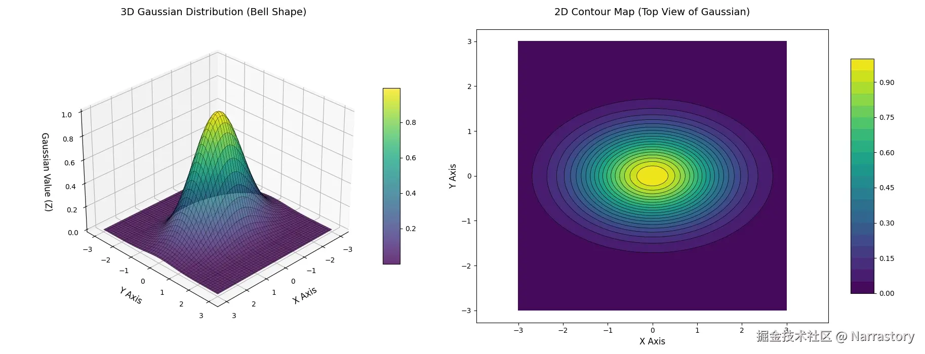
下面的图像展示了一个典型的二维高斯分布（二元正态分布） 的概率密度曲面图。它是一个平滑的钟形曲面 ，其峰值位于均值点 <math xmlns="http://www.w3.org/1998/Math/MathML"> ( μ 1 , μ 2 ) (\mu_1,\mu_2) </math>(μ1,μ2) 处。曲面的"形状"由协方差矩阵 <math xmlns="http://www.w3.org/1998/Math/MathML"> Σ \Sigma </math>Σ 决定。下图清晰地展示了这种对称的钟形结构：

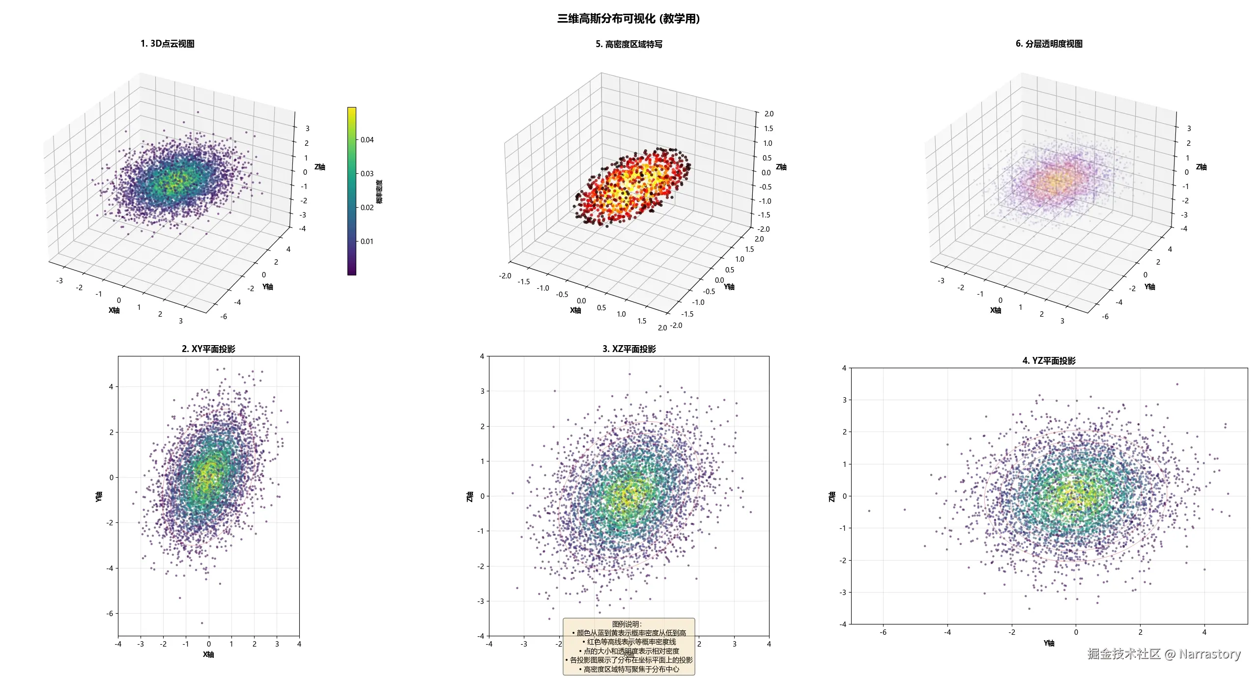
对于三维高斯分布，在三维空间中完整可视化概率密度函数较为困难，因此常用三维点云图来近似表示其分布形态。在下图中，每个点的位置代表一个三维样本，颜色或密度表示该点出现的概率大小。可以看到，样本点密集地分布在均值点附近，并随着距离增加而逐渐稀疏，整体形状大致呈椭球状。这个椭球的朝向与伸展程度，完全由三维协方差矩阵的特征向量和特征值决定。

因此，在数学上， <math xmlns="http://www.w3.org/1998/Math/MathML"> n n </math>n 维高斯分布（多元正态分布）的概率密度函数定义为：
<math xmlns="http://www.w3.org/1998/Math/MathML" display="block"> N ( x ∣ μ , Σ ) = 1 ( 2 π ) n 2 ∣ Σ ∣ 0.5 exp ⁡ ( − ( x − μ ) T Σ − 1 ( x − μ ) 2 ) \mathcal{N}(\mathbf{x}|\boldsymbol{\mu},\Sigma ) = \frac{1}{(2\pi)^{\frac{n}{2} }|\Sigma|^{0.5}}\exp(-\frac{(\mathbf{x}-\boldsymbol{\mu})^{T}\Sigma^{-1}(\mathbf{x}-\boldsymbol{\mu})}{2} ) </math>N(x∣μ,Σ)=(2π)2n∣Σ∣0.51exp(−2(x−μ)TΣ−1(x−μ))

初次见到这个公式可能会觉得复杂，但我们可以这样理解：它本质上是一个多元函数 <math xmlns="http://www.w3.org/1998/Math/MathML"> f ( x 1 , x 2 , ... , x n ) f(x_1, x_2, \dots, x_n) </math>f(x1,x2,...,xn)，其核心结构仍与一维高斯分布相似，只是将标量均值 <math xmlns="http://www.w3.org/1998/Math/MathML"> μ \mu </math>μ 扩展为均值向量 <math xmlns="http://www.w3.org/1998/Math/MathML"> μ \boldsymbol{\mu} </math>μ，并将方差 <math xmlns="http://www.w3.org/1998/Math/MathML"> σ 2 \sigma^2 </math>σ2 推广为协方差矩阵 <math xmlns="http://www.w3.org/1998/Math/MathML"> Σ \Sigma </math>Σ。

式中各符号的含义如下：

<math xmlns="http://www.w3.org/1998/Math/MathML"> x \mathbf{x} </math>x 是 <math xmlns="http://www.w3.org/1998/Math/MathML"> n n </math>n 维数据向量，形状为 <math xmlns="http://www.w3.org/1998/Math/MathML"> n × 1 n \times 1 </math>n×1，表示一个观测样本；
<math xmlns="http://www.w3.org/1998/Math/MathML"> μ \boldsymbol{\mu} </math>μ 是 <math xmlns="http://www.w3.org/1998/Math/MathML"> n n </math>n 维均值向量，形状为 <math xmlns="http://www.w3.org/1998/Math/MathML"> n × 1 n \times 1 </math>n×1，表示各维度上的均值；
<math xmlns="http://www.w3.org/1998/Math/MathML"> Σ \Sigma </math>Σ 是 <math xmlns="http://www.w3.org/1998/Math/MathML"> n × n n \times n </math>n×n 的协方差矩阵（实对称且正定），它决定了分布的形态与方向；
<math xmlns="http://www.w3.org/1998/Math/MathML"> Σ − 1 \Sigma^{-1} </math>Σ−1 是协方差矩阵的逆；
<math xmlns="http://www.w3.org/1998/Math/MathML"> ∣ Σ ∣ |\Sigma| </math>∣Σ∣ 表示协方差矩阵的行列式，用于对整个分布进行归一化。

下面我们用 Python 来实现这个多元高斯分布的概率密度函数：

python 复制代码

import numpy as np
def multivariate_gaussian(x, mu, Sigma):
    """
    计算多元高斯分布的概率密度函数

    参数:
    x: 输入向量, 形状 (n,)
    mu: 均值向量, 形状 (n,)
    Sigma: 协方差矩阵, 形状 (n, n)

    返回:
    概率密度值：标量
    """
    # 1. 计算维度
    n = len(mu)
    # 2. 计算协方差矩阵的行列式
    det_Sigma = np.linalg.det(Sigma)
    # 3. 计算协方差矩阵的逆
    inv_Sigma = np.linalg.inv(Sigma)
    # 4. 计算 x 与 mu 的差值
    diff = x - mu
    # 5. 计算指数部分: (x-μ)^T Σ^(-1) (x-μ)
    exponent = -0.5 * diff.T @ inv_Sigma @ diff
    # 6. 计算归一化系数
    normalization = 1.0 / ((2 * np.pi) ** (n / 2) * np.sqrt(det_Sigma))
    # 7. 计算最终概率密度
    pdf_value = normalization * np.exp(exponent)
    return pdf_value

下面来使用一下这个multivariate_gaussian函数：

python 复制代码

# 均值向量
mu = np.array([0.0, 0.0])
# 协方差矩阵（正定对称）
Sigma = np.array([[1.0, 0.5], 
                  [0.5, 1.0]])
# 测试点
x_test = np.array([0.5, 0.5])
# 计算测试点的概率密度
pdf_value = multivariate_gaussian(x_test, mu, Sigma)
# 输出结果
print(f"概率密度 N(x|μ,Σ): {pdf_value}")

## ====输出====
概率密度 N(x|μ,Σ): 0.1555632781262252

从直观上理解， <math xmlns="http://www.w3.org/1998/Math/MathML"> μ \boldsymbol{\mu} </math>μ 表示数据分布的中心位置， <math xmlns="http://www.w3.org/1998/Math/MathML"> x \mathbf{x} </math>x 是空间中的一个点，概率密度函数 <math xmlns="http://www.w3.org/1998/Math/MathML"> f ( x ) f(\mathbf{x}) </math>f(x) 则反映了该点出现的相对可能性/概率。

然而，为什么一维高斯中的标准差 <math xmlns="http://www.w3.org/1998/Math/MathML"> σ \sigma </math>σ 在多维情况下会扩展为一个协方差矩阵 <math xmlns="http://www.w3.org/1998/Math/MathML"> Σ \Sigma </math>Σ？这是很多初学者感到困惑的地方。
<math xmlns="http://www.w3.org/1998/Math/MathML" display="block"> Σ = [ σ 11 σ 12 ... σ 1 n σ 21 σ 22 ... σ 2 n ⋮ ⋮ ⋱ ⋮ σ n 1 σ n 2 ... σ n n ] , σ i j = σ j i \Sigma = \begin{bmatrix} \sigma_{11} &\sigma_{12} & \dots &\sigma_{1n} \\ \sigma_{21} & \sigma_{22} & \dots & \sigma_{2n}\\ \vdots & \vdots & \ddots & \vdots \\ \sigma_{n1} & \sigma_{n2} & \dots & \sigma_{nn} \end{bmatrix} \space, \space \sigma_{ij} = \sigma_{ji} </math>Σ= σ11σ21⋮σn1σ12σ22⋮σn2......⋱...σ1nσ2n⋮σnn , σij=σji

其实，多维数据不仅在各维度上具有各自的离散程度，不同维度之间还可能存在关联性，从而形成具有特定方向和形状的概率椭球（或超椭球）。协方差矩阵 <math xmlns="http://www.w3.org/1998/Math/MathML"> Σ \Sigma </math>Σ 正是为了完整刻画这种多维结构：

其对角线元素 <math xmlns="http://www.w3.org/1998/Math/MathML"> σ i i \sigma_{ii} </math>σii 表示第 <math xmlns="http://www.w3.org/1998/Math/MathML"> i i </math>i 个维度的方差；
非对角线元素 <math xmlns="http://www.w3.org/1998/Math/MathML"> σ i j \sigma_{ij} </math>σij 表示第 <math xmlns="http://www.w3.org/1998/Math/MathML"> i i </math>i 维与第 <math xmlns="http://www.w3.org/1998/Math/MathML"> j j </math>j 维之间的协方差，描述了两个维度之间的线性相关程度和共同变化趋势。

理解了概率密度函数可以延伸到多维之后，我们可以更准确地重申高斯混合模型的核心思想：混合高斯模型（GMM）是一种强大的概率建模工具，它旨在将任意复杂的 <math xmlns="http://www.w3.org/1998/Math/MathML"> n n </math>n维概率分布 <math xmlns="http://www.w3.org/1998/Math/MathML"> f ( x ) f(\mathbf{x}) </math>f(x)，分解为 <math xmlns="http://www.w3.org/1998/Math/MathML"> k k </math>k个 <math xmlns="http://www.w3.org/1998/Math/MathML"> n n </math>n维高斯分布的加权线性组合。
<math xmlns="http://www.w3.org/1998/Math/MathML" display="block"> f ( x ) = ∑ i = 1 k π i N ( x ∣ μ i , Σ i ) f(\mathbf{x}) = \sum_{i=1}^{k} \pi_{i}\space \mathcal{N}(\mathbf{x}|\boldsymbol{\mu}{i},\Sigma{i}) </math>f(x)=i=1∑kπi N(x∣μi,Σi)

其中， <math xmlns="http://www.w3.org/1998/Math/MathML"> π i \pi_{i} </math>πi表示第 <math xmlns="http://www.w3.org/1998/Math/MathML"> i i </math>i个高斯分布的权重系数，并且满足 <math xmlns="http://www.w3.org/1998/Math/MathML"> π i ≥ 0 , ∑ i = 1 k π i = 1 \pi_{i} \ge 0, \sum_{i=1}^{k} \pi_{i} = 1 </math>πi≥0,∑i=1kπi=1

基于前面介绍的理论基础，现在我们就以二维概率分布 <math xmlns="http://www.w3.org/1998/Math/MathML"> f ( x ) f(\mathbf{x}) </math>f(x) 为例，来可视化演示如何用多个高斯分布对其逼近与分解。

值得注意的是，这类分解并不像泰勒展开那样存在确定的数学解析解 。由于我们面对的是一个由多个高斯成分叠加而成的混合模型，其参数估计问题没有闭式解，通常只能通过迭代优化 的方法寻找似然函数的一个局部最优解。而这个迭代优化方法的名称就是高斯混合模型（GMM）聚类算法

在实际应用中，我们往往无法直接获得真实分布 <math xmlns="http://www.w3.org/1998/Math/MathML"> f ( x ) f(\mathbf{x}) </math>f(x) 的解析形式，而是通过采样获得有限的数据样本。例如，假设我们通过观测采样得到如下数据集：

样本	特征1	特征2
样本1	0.6	1.1
样本2	3.6	2.5
样本3	2.8	3.3
样本4	0.1	2.7
...

将全部数据绘制在二维平面上，可得到如下散点图：

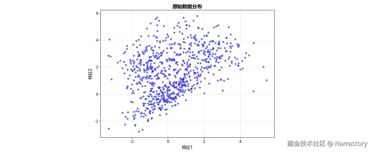
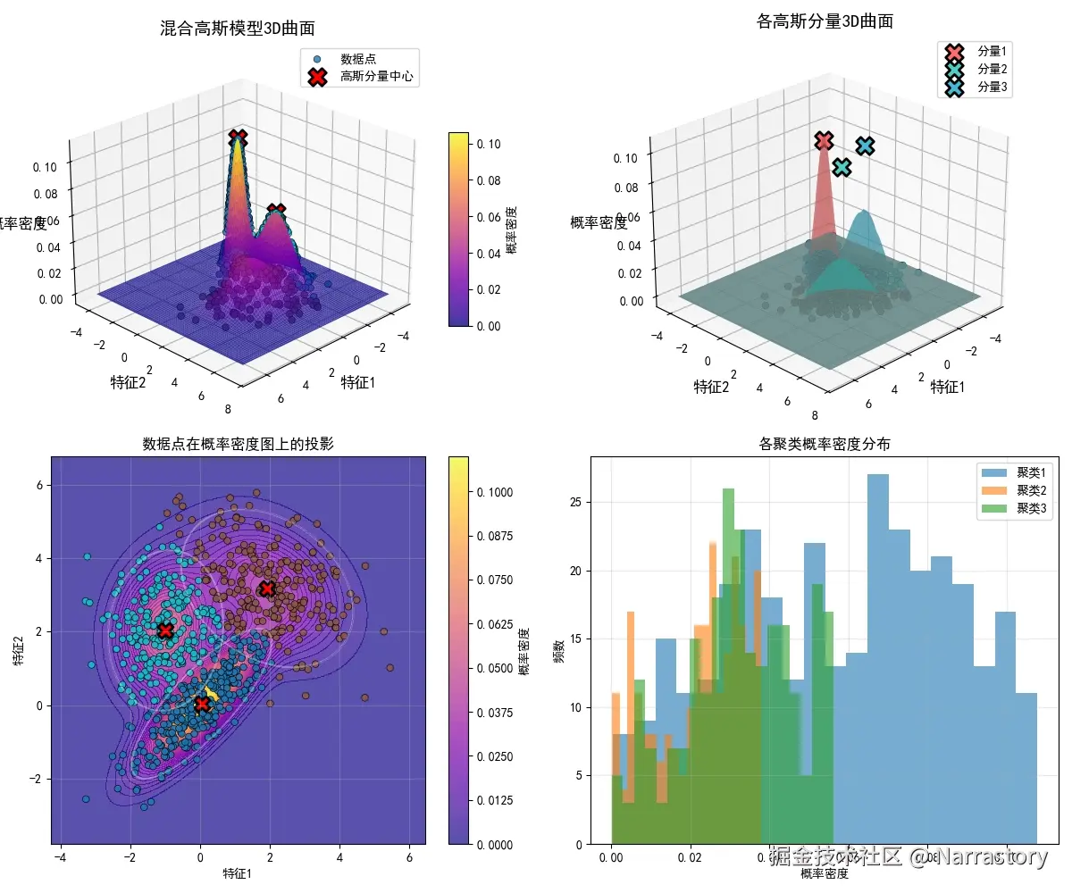
从散点图中虽然难以精确判断数据应由几个二元高斯分布混合而成，但可大致观察到数据似乎围绕三个中心 聚集。因此，我们假设混合成分数 <math xmlns="http://www.w3.org/1998/Math/MathML"> k = 3 k = 3 </math>k=3，并运用 GMM 聚类算法对该分布进行拟合分解。算法运行后，我们得到三个二元高斯分布的参数估计：
<math xmlns="http://www.w3.org/1998/Math/MathML" display="block"> f ( x ) = 0.4 N ( x ∣ [ 0.04 , 0.04 ] , Σ 1 ) + 0.29 N ( x ∣ [ 1.92 , 3.18 ] , Σ 2 ) + 0.31 N ( x ∣ [ − 0.98 , 2.03 ] , Σ 3 ) f(\mathbf{x}) = 0.4 \mathcal{N}(\mathbf{x} \mid [0.04,0.04],\Sigma_1) + 0.29 \mathcal{N}(\mathbf{x} \mid [1.92,3.18],\Sigma_2)+0.31 \mathcal{N}(\mathbf{x} \mid [-0.98,2.03],\Sigma_3) </math>f(x)=0.4N(x∣[0.04,0.04],Σ1)+0.29N(x∣[1.92,3.18],Σ2)+0.31N(x∣[−0.98,2.03],Σ3)
<math xmlns="http://www.w3.org/1998/Math/MathML" display="block"> Σ 1 = [ 1 0.8 0.8 1 ] \Sigma_1 = \begin{bmatrix} 1 & 0.8\\ 0.8 &1 \end{bmatrix} </math>Σ1=[10.80.81]
<math xmlns="http://www.w3.org/1998/Math/MathML" display="block"> Σ 2 = [ 1.5 − 0.6 − 0.6 1.5 ] \Sigma_2 = \begin{bmatrix} 1.5 & -0.6\\ -0.6 &1.5 \end{bmatrix} </math>Σ2=[1.5−0.6−0.61.5]
<math xmlns="http://www.w3.org/1998/Math/MathML" display="block"> Σ 3 = [ 0.8 0 0 0.8 ] \Sigma_3 = \begin{bmatrix} 0.8 & 0\\ 0 &0.8 \end{bmatrix} </math>Σ3=[0.8000.8]

可视化后如下图所示：

接下来，我们将深入讲解GMM聚类算法的数学流程。如果你对下面的数学公式感到头大，也不必担心，你可以直接跳过这一小节，去学习GMM聚类算法的工具库。毕竟在大多数情况下，我们只要会用工具就行了，没必要知道工具是如何运作的。但是如果有能力的话，还是推荐你尝试理解一下，看看别人的设计思想，以后自己设计新算法或进行理论创新时也有个参考。

假设我们有一个包含 <math xmlns="http://www.w3.org/1998/Math/MathML"> m m </math>m 个 <math xmlns="http://www.w3.org/1998/Math/MathML"> n n </math>n 维样本的数据集 <math xmlns="http://www.w3.org/1998/Math/MathML"> X = x ( 1 ) , x ( 2 ) , . . . , x ( m ) \mathbf{X} = {\mathbf{x}^{(1)}, \mathbf{x}^{(2)}, ..., \mathbf{x}^{(m)}} </math>X=x(1),x(2),...,x(m)，可以表示为形状为 <math xmlns="http://www.w3.org/1998/Math/MathML"> ( m , n ) (m, n) </math>(m,n) 的矩阵。我们的目标是将数据分布分解为 <math xmlns="http://www.w3.org/1998/Math/MathML"> k k </math>k 个 <math xmlns="http://www.w3.org/1998/Math/MathML"> n n </math>n 维高斯分布的线性组合。记第 <math xmlns="http://www.w3.org/1998/Math/MathML"> j j </math>j 个高斯分布为 <math xmlns="http://www.w3.org/1998/Math/MathML"> N ( x ∣ μ j , Σ j ) \mathcal{N}(\mathbf{x} \mid \boldsymbol{\mu}_j, \Sigma_j) </math>N(x∣μj,Σj)，其权重为 <math xmlns="http://www.w3.org/1998/Math/MathML"> π j \pi_j </math>πj。 <math xmlns="http://www.w3.org/1998/Math/MathML"> x ( i ) \mathbf{x}^{(i)} </math>x(i)则表示数据集中的第 <math xmlns="http://www.w3.org/1998/Math/MathML"> i i </math>i个样本，形状为 <math xmlns="http://www.w3.org/1998/Math/MathML"> ( n , 1 ) (n,1) </math>(n,1)。

1. 参数初始化

首先需要初始化 <math xmlns="http://www.w3.org/1998/Math/MathML"> k k </math>k 个高斯分布的参数： <math xmlns="http://www.w3.org/1998/Math/MathML"> Σ j , μ j , π j \Sigma_{j},\boldsymbol{\mu}{j},\pi{j} </math>Σj,μj,πj 。完全随机初始化 虽然理论上可行，但实践中容易导致收敛缓慢或陷入较差的局部最优。因此，通常采用K-means聚类的结果进行初始化：

用K-means将数据划分为 <math xmlns="http://www.w3.org/1998/Math/MathML"> k k </math>k 个簇
以每个簇的样本均值作为 <math xmlns="http://www.w3.org/1998/Math/MathML"> μ j \boldsymbol{\mu}_j </math>μj 的初始值
以每个簇的样本协方差作为 <math xmlns="http://www.w3.org/1998/Math/MathML"> Σ j \Sigma_j </math>Σj 的初始值
以每个簇的样本比例作为 <math xmlns="http://www.w3.org/1998/Math/MathML"> π j \pi_j </math>πj 的初始值

2. E步：计算隶属度

然后求出每一个样本 <math xmlns="http://www.w3.org/1998/Math/MathML"> x ( i ) \mathbf{x}^{(i)} </math>x(i) 对应的每一个高斯分布 <math xmlns="http://www.w3.org/1998/Math/MathML"> j j </math>j 的隶属度 <math xmlns="http://www.w3.org/1998/Math/MathML"> γ j ( i ) \gamma_{j}^{(i)} </math>γj(i)（标量），即第 <math xmlns="http://www.w3.org/1998/Math/MathML"> i i </math>i 个数据属于第 <math xmlns="http://www.w3.org/1998/Math/MathML"> j j </math>j 个高斯分布的程度，计算方式如下
<math xmlns="http://www.w3.org/1998/Math/MathML" display="block"> γ j ( i ) = π j N ( x ( i ) ∣ μ j , Σ j ) ∑ l = 1 k π l N ( x ( i ) ∣ μ l , Σ l ) \gamma_{j}^{(i)} = \frac{\pi_{j} \space \mathcal{N}(\mathbf{x}^{(i)}\mid \boldsymbol{\mu}{j},\Sigma{j})}{ {\textstyle \sum_{l=1}^{k}} \pi_{l} \space \mathcal{N}(\mathbf{x}^{(i)}\mid \boldsymbol{\mu}{l},\Sigma{l})} </math>γj(i)=∑l=1kπl N(x(i)∣μl,Σl)πj N(x(i)∣μj,Σj)

3. M步：更新参数

基于E步计算出的责任，我们更新每个高斯成分的参数

更新均值 <math xmlns="http://www.w3.org/1998/Math/MathML"> μ j \boldsymbol{\mu}_j </math>μj（向量）：

<math xmlns="http://www.w3.org/1998/Math/MathML" display="block"> μ j = ∑ i = 1 m γ j ( i ) x ( i ) ∑ i = 1 m γ j ( i ) \boldsymbol{\mu}{j} = \frac{{\textstyle \sum{i=1}^{m}} \gamma_{j}^{(i)}\mathbf{x}^{(i)}}{ {\textstyle \sum_{i=1}^{m}} \gamma_{j}^{(i)}} </math>μj=∑i=1mγj(i)∑i=1mγj(i)x(i)

更新混合权重 <math xmlns="http://www.w3.org/1998/Math/MathML"> π j \pi_j </math>πj（标量）

<math xmlns="http://www.w3.org/1998/Math/MathML" display="block"> π j = 1 m ∑ i = 1 m γ j ( i ) \pi_{j} = \frac{1}{m} \sum_{i=1}^{m} \gamma_{j}^{(i)} </math>πj=m1i=1∑mγj(i)

更新协方差 <math xmlns="http://www.w3.org/1998/Math/MathML"> Σ j \Sigma_j </math>Σj（矩阵）

<math xmlns="http://www.w3.org/1998/Math/MathML" display="block"> Σ j = ∑ i = 1 m γ j ( i ) ( x ( i ) − μ j ) ( x ( i ) − μ j ) T ∑ i = 1 m γ j ( i ) \Sigma_{j} = \frac{{\textstyle \sum_{i=1}^{m}} \gamma_{j}^{(i)}(\mathbf{x}^{(i)}-\boldsymbol{\mu}{j})(\mathbf{x}^{(i)}-\boldsymbol{\mu}{j})^{T}}{ {\textstyle \sum_{i=1}^{m}} \gamma_{j}^{(i)}} </math>Σj=∑i=1mγj(i)∑i=1mγj(i)(x(i)−μj)(x(i)−μj)T

重复执行E步和M步，不断更新 <math xmlns="http://www.w3.org/1998/Math/MathML"> Σ j , μ j , π j \Sigma_{j},\boldsymbol{\mu}{j},\pi{j} </math>Σj,μj,πj，通常迭代 <math xmlns="http://www.w3.org/1998/Math/MathML"> 20 20 </math>20- <math xmlns="http://www.w3.org/1998/Math/MathML"> 100 100 </math>100 次，最终会收敛到一个局部最优解。

最终我们得到了的 <math xmlns="http://www.w3.org/1998/Math/MathML"> k k </math>k 个高斯分布 <math xmlns="http://www.w3.org/1998/Math/MathML"> N ( x ∣ μ j , Σ j ) \mathcal{N}(\mathbf{x} \mid \boldsymbol{\mu}j, \Sigma_j) </math>N(x∣μj,Σj)及其权重 <math xmlns="http://www.w3.org/1998/Math/MathML"> π j \pi{j} </math>πj，以及每个样本对各个高斯分布的隶属度 <math xmlns="http://www.w3.org/1998/Math/MathML"> γ j ( i ) \gamma_j^{(i)} </math>γj(i)。这些参数完整刻画了所有数据的混合分布。

如果你理解了上述数学流程，那么即使不使用现成的GMM库，仅用Python和NumPy也能实现一个完整的GMM聚类算法。下面将展示如何调用成熟的机器学习库来使用GMM算法。

首先，确保已安装必要的Python库。如果尚未安装Scikit-learn，可通过以下命令安装：

bash 复制代码

pip install scikit-learn

为了演示GMM算法的应用，我们需要一个合适的数据集。因为没有现成的真实数据集，这里就使用make_blobs函数生成一个随机的合成数据集。这个函数特别适合生成符合混合高斯分布的数据，因为它本身就是通过叠加多个高斯分布来创建数据的。

python 复制代码

import numpy as np
from sklearn.datasets import make_blobs

# 生成示例数据
# n_samples: 样本数量（500个）
# n_features: 特征维度（3维）
# centers: 聚类中心数量（4个）
# cluster_std: 每个簇的标准差（控制簇的紧密度）
# random_state: 随机种子，确保结果可复现
dataset, _ = make_blobs(
    n_samples=500, 
    n_features=3, 
    centers=4, 
    cluster_std=1.8, 
    random_state=3212
)

print(dataset.shape)	# 查看数据的形状
print(dataset[:10])	# 查看前10个数据

# === 输出 ===
(500,3)

[[ -2.2167599 ,  -7.11603166,   3.99062792],
 [ -1.90878361,  -4.10948361,   5.1927847 ],
 [ -1.96540003,  -6.17016357,   2.79308236],
 [ -1.90406637,   0.73862831, -10.0718729 ],
 [ -9.08810591,  -6.24574275,  -1.24825942],
 [ -6.03737854,  -6.50248559,   2.76654161],
 [ -1.46453584,  -8.28078741,   2.93290504],
 [ -1.87337298,  -5.32761017,   3.79653868],
 [  6.21321387,   4.5978286 ,  -5.75274046],
 [-10.68329327, -10.08210729,  -1.48406785]]

这段代码生成了一个包含500个样本、3个特征的数据集，这些样本来自4个不同的高斯分布。每个分布的中心位置由centers参数控制，而cluster_std参数决定了每个分布的离散程度。

接下来，我们使用Scikit-learn的GaussianMixture类来定义GMM模型。创建模型时需要设置多个重要参数，每个参数都对模型性能有直接影响：

python 复制代码

from sklearn.mixture import GaussianMixture

# 创建GMM模型实例
gmm = GaussianMixture(
    n_components=4,           # ! 要识别的聚类数量（高斯分布个数）
    covariance_type="full",   # 协方差矩阵类型：完全协方差（每个成分有自己的任意协方差矩阵）
    tol=1e-3,                 # 收敛阈值：当对数似然增益小于此值时停止迭代
    max_iter=50,              # ! 最大迭代次数：EM算法的最大迭代轮数
    init_params="kmeans",     # 初始化方法：使用K-means进行参数初始化（比随机初始化更稳定）
    random_state=42,          # 随机种子：确保结果可重复
)

# 训练GMM模型
gmm.fit(dataset)
# x

print(gmm.weights_)	# 获取每个高斯分布的权重
print(gmm.means_)	# 获取每个高斯分布的均值向量
print(gmm.covariances_.shape)	# 获取各高斯成分的协方差矩阵形状
print(gmm.covariances_[0])	# 查看第一个高斯成分的协方差矩阵

# === 输出 ===

# 分别是第0个，第1个，第2个，第3个高斯分布的权重
[0.25001436, 0.25      , 0.23822018, 0.26176546]

# 分别是第0个，第1个，第2个，第3个高斯分布的均值向量 mu
[[-9.27389593, -7.07418061, -0.82308003],
 [ 2.60201839,  3.72587996, -8.02382928],
 [-5.24683692, -7.48695937,  1.07606264],
 [-1.02626245, -6.35110703,  4.6423531 ]]

# 4个3x3的协方差矩阵
(4, 3, 3)

# 第一个高斯成分的协方差矩阵
[[ 3.56369354,  0.33917216, -0.19620971],
 [ 0.33917216,  3.24354619, -0.17032308],
 [-0.19620971, -0.17032308,  2.71638609]]

训练完成后，我们可以使用模型进行预测和概率计算：

python 复制代码

# 创建测试样本
test_samples = np.array([
    [1.0, 4.1, 3.1],    # 测试样本1
    [-8.0, -6.0, -0.5], # 测试样本2
    [3.0, 4.0, -7.0],   # 测试样本3
    [-2.0, -6.0, 4.0]   # 测试样本4
])

# 预测每个样本最可能属于哪个高斯成分
print(gmm.predict(test_samples)) 

# === 输出 ===
[3, 0, 1, 3]
# 表明了测试样本1属于第3个高斯分布，测试样本2属于第0个高斯分布，...

以上就是混合高斯模型的所有内容了，对于看到这里的你，恭喜你，你现在已经掌握了这一强大的概率建模工具！

回想我最初学习机器学习时，常常是听说一个方法就去学，但学完却不知道它究竟能解决什么问题，学了跟没学一样，这或许是很多人共同的学习经历。而真正的理解，往往发生在你将一个抽象算法与一个具体问题联系起来的那一刻。

举个有趣的例子吧，如今智能手机上的运动App都非常智能，你只要把手机揣在兜里或者拿在手上，然后开始运动，它就能通过分析手机的各种传感器数据，来自动推理出你当前的运动状态，是在步行、跑步、骑行 ，还是静止。我想你会好奇，它是怎么知道我们的运动状态的。

相信你在了解了混合高斯分布后就会理解它的原理：每个传感器（如加速度计、陀螺仪、GPS等）收集到的数据就是一个特征，传感器在每个时刻都会收集到数据。我们可以在一段时间内每隔0.5s采样一次所有传感器的数据，然后对这一段时间内的数据进行GMM聚类分析。将其分解成多个多元高斯分布，通过分析比对不同的高斯分布，就能推断出你的运动状态。如果你感兴趣，完全可以自己去尝试一下。