文章目录
- [1. 本节整体内容](#1. 本节整体内容)
-
- [1.1 概要](#1.1 概要)
- [1.2 引子(一些快速计算例子)](#1.2 引子(一些快速计算例子))
- [1.3 推荐transformer读物](#1.3 推荐transformer读物)
- [2. Memory accounting](#2. Memory accounting)
-
- [2.1 tensors_basics](#2.1 tensors_basics)
- [2.2 tensors_memory](#2.2 tensors_memory)
-
- [2.2.1 float32(FP32)](#2.2.1 float32(FP32))
- [2.2.2 float16(FP16)](#2.2.2 float16(FP16))
- [2.2.3 bfloat16(BF16)](#2.2.3 bfloat16(BF16))
- [2.2.4 fp32,fp16,bf16表示范围对比](#2.2.4 fp32,fp16,bf16表示范围对比)
- [2.2.5 fp8](#2.2.5 fp8)
- [3. Compute accounting](#3. Compute accounting)
-
- [3.1 tensors_on_gpus()](#3.1 tensors_on_gpus())
- [3.2 tensor_operations()](#3.2 tensor_operations())
-
- [3.2.1 tensor_storage()](#3.2.1 tensor_storage())
- [3.2.2 tensor_slicing()](#3.2.2 tensor_slicing())
- [3.2.3 tensor_elementwise()](#3.2.3 tensor_elementwise())
- [3.2.4 tensor_matmul()](#3.2.4 tensor_matmul())
- [3.3 tensor_einops()](#3.3 tensor_einops())
-
- [3.3.1 使用einops的motivation](#3.3.1 使用einops的motivation)
- [3.3.2 jaxtyping类型注释](#3.3.2 jaxtyping类型注释)
- [3.3.3 einops使用](#3.3.3 einops使用)
-
- [3.3.3.1 einops的einsum和torch.einsum](#3.3.3.1 einops的einsum和torch.einsum)
- [3.3.3.2 einops的reduce](#3.3.3.2 einops的reduce)
- [3.3.3.3 einops的rearrange](#3.3.3.3 einops的rearrange)
- [3.4 tensor_operations_flops()](#3.4 tensor_operations_flops())
-
- [3.4.1 基本介绍( FLOPs vs. FLOP/s vs FLOPS)](#3.4.1 基本介绍( FLOPs vs. FLOP/s vs FLOPS))
- [3.4.2 直观感受](#3.4.2 直观感受)
- [3.4.3 以线性模型为例计算`矩阵乘法的运算量`](#3.4.3 以线性模型为例计算
矩阵乘法的运算量) - [3.4.4 其他矩阵操作的运算量](#3.4.4 其他矩阵操作的运算量)
- [3.4.5 推广到transformers的计算量](#3.4.5 推广到transformers的计算量)
- [3.4.6 理论计算速度和实际计算速度](#3.4.6 理论计算速度和实际计算速度)
- [3.4.7 MFU](#3.4.7 MFU)
- [3.4.X 总结](#3.4.X 总结)
- [3.5 gradients_basics()](#3.5 gradients_basics())
- [3.6 gradients_flops()](#3.6 gradients_flops())
- [4. Model](#4. Model)
-
- [4.1 module_parameters()](#4.1 module_parameters())
- [4.2 custom_model()](#4.2 custom_model())
- [4.3 Training loop and best practices](#4.3 Training loop and best practices)
-
- [4.3.1 note_about_randomness](#4.3.1 note_about_randomness)
- [4.3.2 data_loading()](#4.3.2 data_loading())
- [4.4 optimizer()](#4.4 optimizer())
-
- [4.4.1 自定义优化器+单步优化过程](#4.4.1 自定义优化器+单步优化过程)
- [4.4.2 优化器的存储占用(Optimizer Memory)](#4.4.2 优化器的存储占用(Optimizer Memory))
- [4.5 前向+反向运算总结](#4.5 前向+反向运算总结)
-
- [4.5.1 简单的线性层示例](#4.5.1 简单的线性层示例)
- [4.5.2 Transformers](#4.5.2 Transformers)
- [4.5 train_loop()](#4.5 train_loop())
- [4.6 checkpointing()](#4.6 checkpointing())
- [4.7 mixed_precision_training()](#4.7 mixed_precision_training())
- X.其他
-
- [X. 1. 加减乘除都是用加法器实现的?](#X. 1. 加减乘除都是用加法器实现的?)
- [X.2 动量类的优化算法](#X.2 动量类的优化算法)
-
- [1. 带momentum的SGD](#1. 带momentum的SGD)
- [2. AdaGrad](#2. AdaGrad)
链接:
- b站视频链接: 斯坦福CS336:大模型从0到1|第二讲:pytorch手把手搭建LLM【中英双语】
- 课程ppt:
1. 本节整体内容
1.1 概要
- 学习训练一个模型需要的pytorch的所有原语(primitives)
- 自底向上,从tensors(张量)到models(模型)到optimizers(优化器)到training loop(训练)
- 构建过程中会额外注意 efficiency,即:如何有效利用资源,主要就是两类资源:
- 内存:Memory (GB)------Memory accounting
- 计算:Compute (FLOPs)------Compute accounting
1.2 引子(一些快速计算例子)
1. Question: How long would it take to train a 70B parameter model on 15T tokens on 1024 H100s?
- 在1024个H100显卡上,用15T的数据,训练一个70B/700亿参数(默认密集型)的模型要多久?
python
In [2]: import math
In [3]: 8e2   # 在 Python 中,8e2 是一种科学计数法(scientific notation)的表示方式,用来简洁地表示非常大或非常小的数字。
Out[3]: 800.0

# from facts import a100_flop_per_sec, h100_flop_per_sec
# facts内容就是以下两个常数,
# https://github.com/stanford-cs336/spring2025-lectures/blob/main/facts.py

# https://www.nvidia.com/content/dam/en-zz/Solutions/Data-Center/a100/pdf/nvidia-a100-datasheet-us-nvidia-1758950-r4-web.pdf
a100_flop_per_sec = 312e12  # 312 TFLOP/s
# https://resources.nvidia.com/en-us-tensor-core/nvidia-tensor-core-gpu-datasheet
h100_flop_per_sec = 1979e12 / 2  # 1979 TFLOP/s with sparsity (BF16 tensor core)

# 1. 计算训练所需要的总浮点运算次数 = 6*参数量*tokens数量
total_flops = 6*70e9*15e12    # 6.3e+24
assert h100_flop_per_sec == 1979e12 / 2
mfu = 0.5
# 2. 每天可以计算的flops
flops_per_day = h100_flop_per_sec * mfu * 1024 * 60 * 60 * 24   # 4.37723136e+22
# 3. 训练需要的天数
days = total_flops / flops_per_day # 143.92659381842682其中,关于mfu:
- 在大模型(特别是大语言模型,LLM)的训练和推理领域,MFU 是 Model FLOPs Utilization(模型浮点运算利用率)的缩写。
- 它是一个衡量硬件计算效率的关键指标,用于评估在训练或推理过程中,实际用于模型有效计算的浮点运算(FLOPs)占硬件理论峰值计算能力的比例。
- M F U = 硬件理论峰值 F L O P s 模型每秒实际执行的有效 F L O P s MFU= \frac{硬件理论峰值 FLOPs}{模型每秒实际执行的有效 FLOPs} MFU=模型每秒实际执行的有效FLOPs硬件理论峰值FLOPs
详见: ****
参考:
- Product Specifications
- FP16 Tensor Core* 1,979 teraFLOPS, 万亿(tera-)
2. Question: What's the largest model that can you can train on 8 H100s using AdamW (naively)?
- 使用原生的
AdamW优化器,可以在8个H100上训练多大的模型?
python
# 以下计算单位都是字节
h100_bytes = 80e9   # H100是80GB的显存 1G = e3MB = e6KB = e9B(字节)
bytes_per_parameter = 4 + 4 + (4 + 4)  # 每个参数(parameters), 参数的梯度(gradients)以及优化器状态(optimizer state)
num_parameters = (h100_bytes * 8) / bytes_per_parameter   # 8个H100显卡
num_parameters # 40000000000.0  4e10 400亿

# 注意,这里是非常粗略的计算,没有考虑激活值等内容
# 激活值取决于batch size和 sequence length
1.3 推荐transformer读物
这里不会细讲transformer,下节讲,但是这里可以推荐一些相关内容
注意:
- 这里会使用比transformer更简单的模型
- 因为本节的目的是学会pytorch原语,以及资源计算~
2. Memory accounting
2.1 tensors_basics
张量Tensors是存储所有东西的基础,parameters, gradients, optimizer state, data, activations这些,都是以张量这种数据格式存在和存储的。Pytorch tensors
python
# 创建张量的方式
x = torch.tensor([[1., 2, 3], [4, 5, 6]])
x = torch.zeros(4, 8)  # 4x8 matrix of all zeros
x = torch.ones(4, 8)  # 4x8 matrix of all ones
x = torch.randn(4, 8)  # 4x8 matrix of iid Normal(0, 1) samples

# 创建但不初始化
x = torch.empty(4, 8)  # 4x8 matrix of uninitialized values

# 也可以直接用一些分布来快速赋值,截断的正态分布
# https://docs.pytorch.org/docs/stable/nn.init.html#torch.nn.init.trunc_normal_
#
nn.init.trunc_normal_(x, mean=0, std=1, a=-2, b=2)
2.2 tensors_memory
在深度学习中,大部分用到的张量,比如:参数,梯度,优化器状态,激活值等,都是作为浮点数进行存储的。
2.2.1 float32(FP32)
关于浮点数的存储,最常见的就是float 32(最开始学高级编程语言,C语言默认的浮点数就是4字节,即32位浮点数), 下图自wiki: Single-precision floating-point format(单精度浮点数)
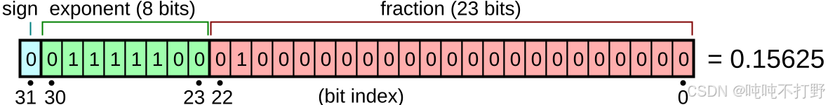
可以看一下《计算机系统结构》课/书里关于数据表示的内容。(现代的大部分计算机都引入了浮点数据表示方式。在<<汇编语言程序设计>>课中, 大家已经学习了浮点数的格式及其用法,在《计算机组成原理》课中, 已经学习了浮点数的运算方法(加减、乘、除等)及运算器的工作原理等, 《计算机系统结构》将重点介绍 浮点数据的分析和设计方法。)但是书里东西写的太复杂了,还是直接看wiki上给的例子吧。
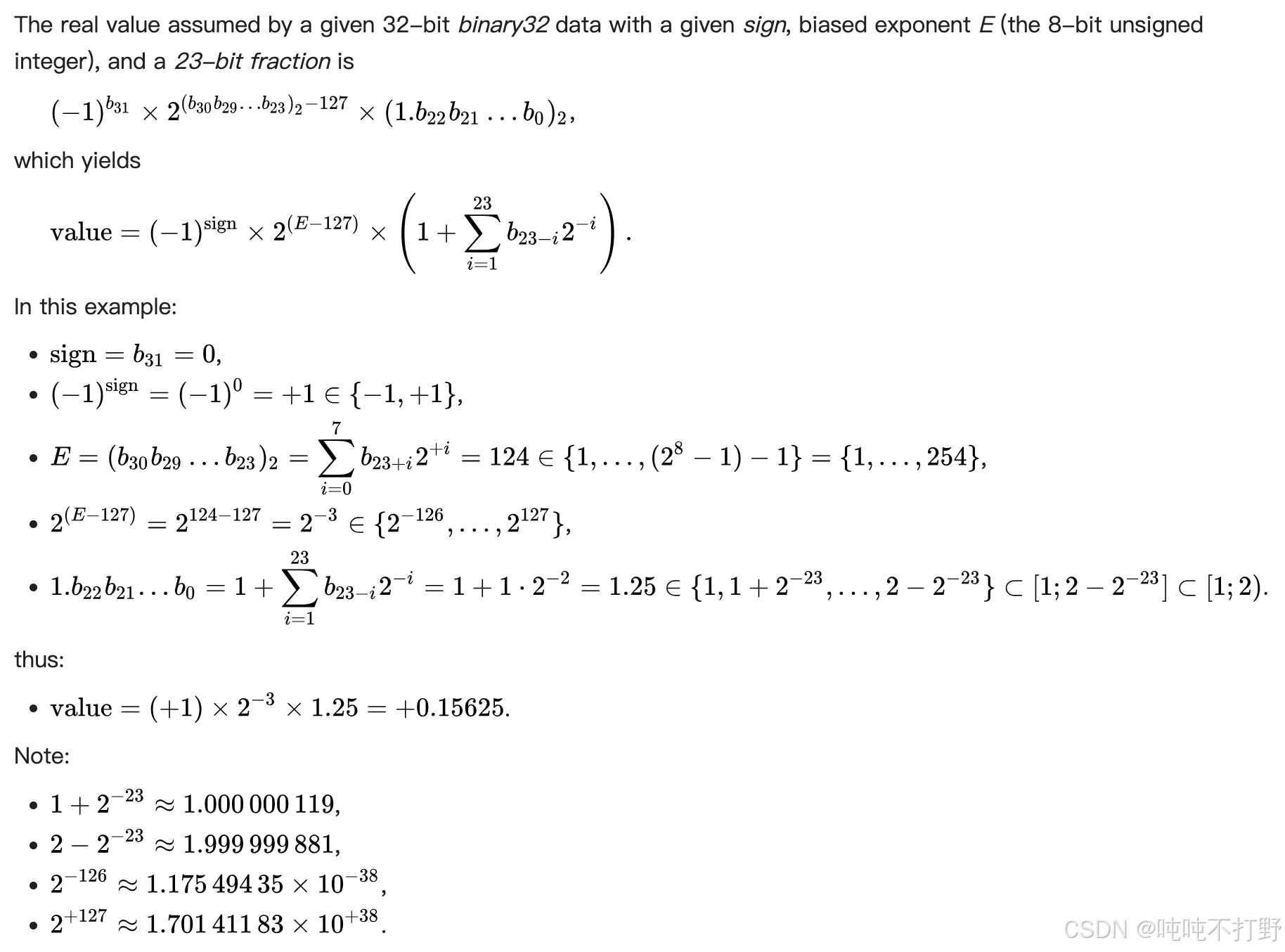
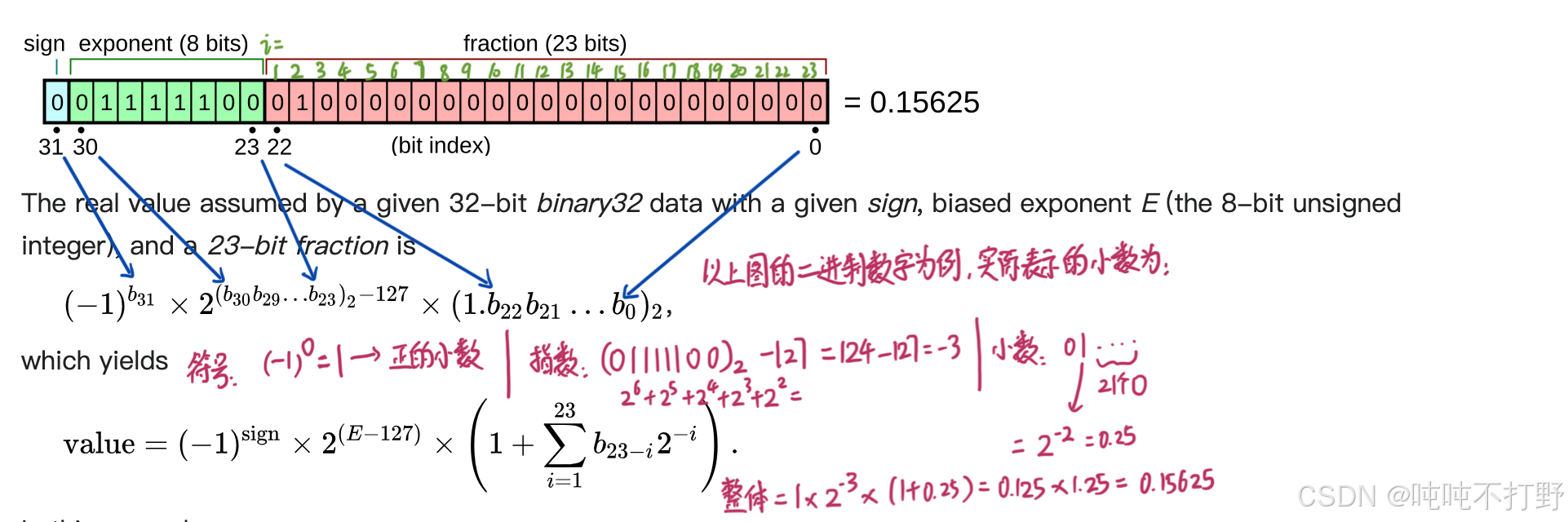
上图的浮点数表示,对应的真值,计算过程为:
手写笔记标注:
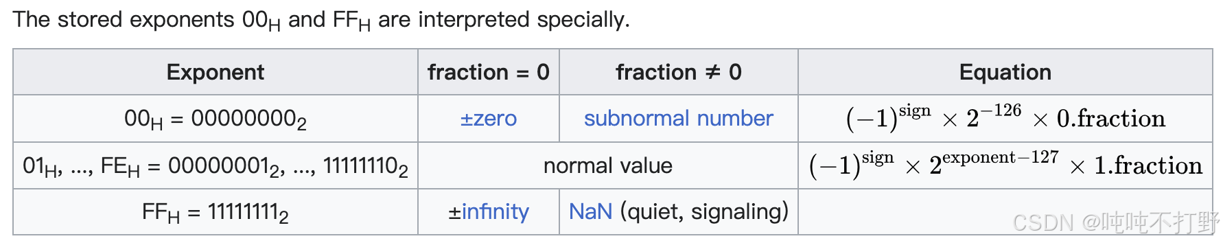
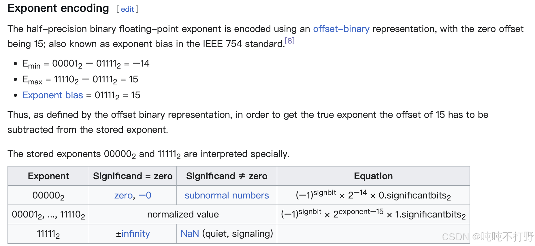
单精度二进制浮点数的指数采用偏移二进制(offset-binary)表示法进行编码,其零偏移值为127;在IEEE 754标准中,这也被称为指数偏置(exponent bias)。
所以当指数是全0或者全1的时候,属于特殊情况
A signed 32-bit integer variable has a maximum value of 2 31 − 1 = 2 , 147 , 483 , 647 2^{31 }− 1 = 2,147,483,647 231−1=2,147,483,647, whereas an IEEE 754 32-bit base-2 floating-point variable has a maximum value of ( 2 − 2 − 23 ) × 2 127 ≈ 3.4028235 × 10 38 (2 − 2^{−23})× 2^{127} ≈ 3.4028235 × 10^{38} (2−2−23)×2127≈3.4028235×1038
The minimum positive normal value is 2 − 126 ≈ 1.18 × 10 − 38 2^{-126}≈ 1.18\times 10^{-38} 2−126≈1.18×10−38 and the minimum positive (subnormal) value is 2 − 149 = 2 − 126 × 2 − 23 ≈ 1.4 × 10 − 45 2^{-149}=2^{-126}\times2^{-23}≈ 1.4\times 10^{-45} 2−149=2−126×2−23≈1.4×10−45
所以32位浮点数可以表示的范围是: 1.4 × 10 − 45 , 3.4028235 × 10 38 1.4\\times 10\^{-45}, 3.4028235 × 10\^{38} 1.4×10−45,3.4028235×1038
一个32位的单精度浮点数,由以下三部分组成:
- 1个符号位, sign
- 8个指数/阶数位, exponent: 提供动态范围
- 23个尾数位,fraction:提供数值精度
float32数据类型,也被表示为FP32,或者称为 单精度(Single precision)
- float32是计算机领域的金标准(gold standard), 默认大部分计算都是以float32进行的,
- 也有人称之为 full precision, 全精度,这个说法不是很准确;如果你跟科学计算领域的人说全精度,就不合适,因为科学计算的人一般是double(双精度浮点数)起步,float64位,例如:MATLAB 的默认数值类型为 double
数据占用内存很好计算,对于张量来说,就是张量里含有多少个值,以及每个值的数据类型,例如:
python
import torch
def get_memory_usage(x: torch.Tensor):
    return x.numel() * x.element_size()

x = torch.zeros(4, 8)  # @inspect x
assert x.dtype == torch.float32  # Default type
assert x.numel() == 4 * 8
assert x.element_size() == 4  # Float is 4 bytes
assert get_memory_usage(x) == 4 * 8 * 4  # 128 bytes

# GPT-3的feedforward layer层的一个矩阵
assert get_memory_usage(torch.empty(12288 * 4, 12288)) == 2304 * 1024 * 1024  # 2.3 GB
2.2.2 float16(FP16)
数据精度小一点,存储空间就占据小一点,算的还快一点
Half-precision floating-point format
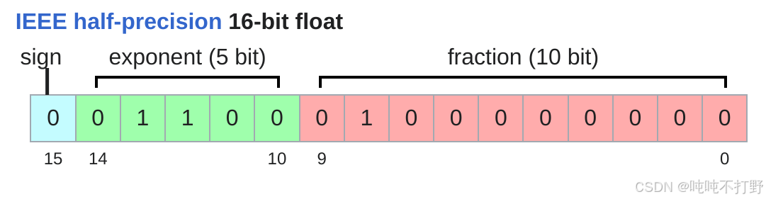
半精度浮点数,FP16,比float32需要的4字节存储,减少了一半
- 1个符号位
- 5个指数/阶数位(比float32的8位少了3个)
- 10个尾数位(比float32的23位少了10个)
python
import torch

x = torch.zeros(4, 8, dtype=torch.float16)
print(x)
assert x.element_size() == 2
# tensor([[0., 0., 0., 0., 0., 0., 0., 0.],
#        [0., 0., 0., 0., 0., 0., 0., 0.],
#        [0., 0., 0., 0., 0., 0., 0., 0.],
#        [0., 0., 0., 0., 0., 0., 0., 0.]], dtype=torch.float16)

x = torch.tensor([1e-8], dtype=torch.float16)
print(x)
assert x == 0  # Underflow/Overflow 下/上溢
# tensor([0.], dtype=torch.float16)
FP16这种数据格式的缺点在于:可以表示的动态范围比较有限。无法表示很大或者很小的数字。
The minimum strictly positive (subnormal) value is 2 − 24 = 2 − 14 × 2 − 10 ≈ 5.96 × 10 − 8 2^{-24}=2^{-14}\times2^{-10}≈ 5.96\times 10^{-8} 2−24=2−14×2−10≈5.96×10⁻⁸ The minimum positive normal value is 2 − 14 ≈ 6.1 × 10 − 5 2^{-14}≈ 6.1\times 10^{-5} 2−14≈6.1×10⁻⁵
The maximum representable value is ( 2 − 2 − 10 ) × 2 15 = 65504 (2−2^{−10}) × 2^{15} = 65504 (2−2−10)×215=65504
因此,如果训练的是个很小的模型,可能还好;但是如果是有很多矩阵,涉及多次连乘的大模型的训练,就很容易出现下溢,导致训练不稳定(出现NaN或者0)。
2.2.3 bfloat16(BF16)
为了解决float16动态范围小的问题,引入了bf16,wiki-bfloat16 floating-point format
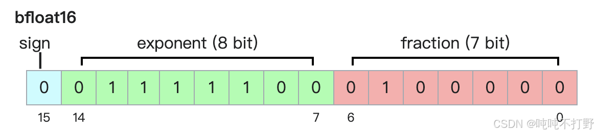
bfloat16 格式,
- 是
Google Brain于2018年提出的解决float16动态范围小的问题的一种数据格式。 - 对于深度学习来说,更关注动态范围,也就是小数的scale,矩阵连乘会导致exp越来越极端;而不是更关注小数的精度(fraction)
- 因此,bfloat16压缩了float16的fraction部分的位数,扩大了exponent部分的位数
- 由此,bfloat16使用float16相同的存储空间,但表示了FP32的动态范围
python
import torch
x = torch.tensor([1e-8], dtype=torch.bfloat16)
print(x)
# tensor([1.0012e-08], dtype=torch.bfloat16)
assert x != 0 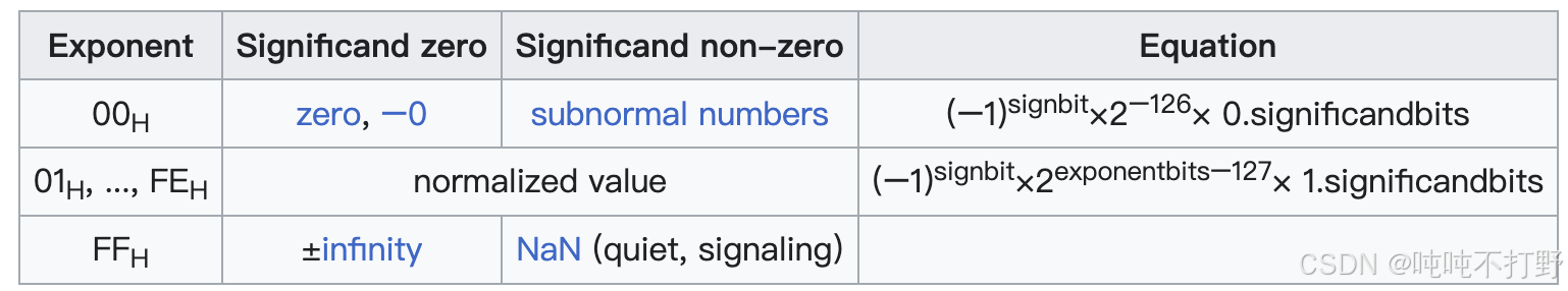
The maximum positive finite value of a normal bfloat16 number is ( 2 8 − 1 ) × 2 − 7 × 2 127 ≈ 3.38953139 × 10 38 (2^8 − 1) × 2^{−7} × 2^{127} ≈ 3.38953139 × 10^{38} (28−1)×2−7×2127≈3.38953139×1038, slightly below ( 2 24 − 1 ) × 2 − 23 × 2 127 = 3.4028235 × 10 38 (2^{24} − 1) × 2^{−23} × 2^{127} = 3.4028235 × 10^{38} (224−1)×2−23×2127=3.4028235×1038, the max finite positive value representable in single precision.
The minimum positive normal value is 2 − 126 ≈ 1.18 × 10 − 38 2^{−126} ≈ 1.18 × 10^{−38} 2−126≈1.18×10−38 and the minimum positive (subnormal) value is 2 − 126 − 7 = 2 − 133 ≈ 9.2 × 10 − 41 2^{−126−7} = 2^{−133} ≈ 9.2 × 10^{−41} 2−126−7=2−133≈9.2×10−41.
bf16的其他说明:
- 是一种截短的 IEEE 754 单精度 32 位浮点数格式,能够快速地与 IEEE 754 单精度 32 位浮点数相互转换;在转换为 bfloat16 格式时,指数位保持不变,而尾数字段则可通过截断(即向零舍入)或其他舍入机制进行缩减,此处暂不考虑 NaN 的特殊情况。
- 保留指数位可维持 32 位浮点数的数值范围,约为 (10^{-38}) 到 (3 \times 10^{38})。
2.2.4 fp32,fp16,bf16表示范围对比
python
import torch
float32_info = torch.finfo(torch.float32)
print(float32_info)
# finfo(resolution=1e-06, min=-3.40282e+38, max=3.40282e+38, eps=1.19209e-07, smallest_normal=1.17549e-38, tiny=1.17549e-38, dtype=float32)
float16_info = torch.finfo(torch.float16)
print(float16_info)
# finfo(resolution=0.001, min=-65504, max=65504, eps=0.000976562, smallest_normal=6.10352e-05, tiny=6.10352e-05, dtype=float16)
bfloat16_info = torch.finfo(torch.bfloat16)
print(bfloat16_info)
# finfo(resolution=0.01, min=-3.38953e+38, max=3.38953e+38, eps=0.0078125, smallest_normal=1.17549e-38, tiny=1.17549e-38, dtype=bfloat16)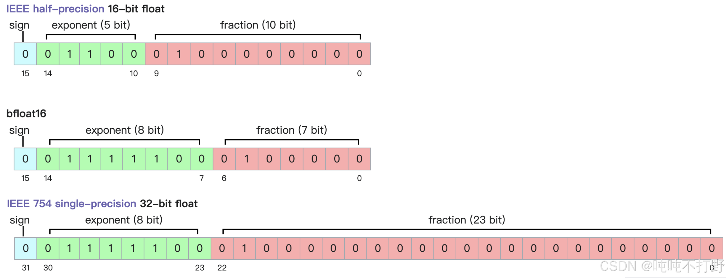
| type | minimum strictly positive (subnormal) | minimum positive normal | maximum |
|---|---|---|---|
| fp32 | 2 − 149 = 2 − 126 × 2 − 23 ≈ 1.4 × 10 − 45 2^{-149}=2^{-126}\times2^{-23}≈ 1.4\times 10^{-45} 2−149=2−126×2−23≈1.4×10−45 | 2 − 126 ≈ 1.18 × 10 − 38 2^{-126}≈ 1.18\times 10^{-38} 2−126≈1.18×10−38 | ( 2 24 − 1 ) × 2 − 23 × 2 127 = 3.4028235 × 10 38 (2^{24} − 1) × 2^{−23} × 2^{127} = 3.4028235 × 10^{38} (224−1)×2−23×2127=3.4028235×1038 |
| fp16 | 2 − 24 = 2 − 14 × 2 − 10 ≈ 5.96 × 10 − 8 2^{-24}=2^{-14}\times2^{-10}≈ 5.96\times 10^{-8} 2−24=2−14×2−10≈5.96×10⁻⁸ | 2 − 14 ≈ 6.1 × 10 − 5 2^{-14}≈ 6.1\times 10^{-5} 2−14≈6.1×10⁻⁵ | ( 2 − 2 − 10 ) × 2 15 = 65504 (2−2^{−10}) × 2^{15} = 65504 (2−2−10)×215=65504 |
| bf16 | 2 − 126 − 7 = 2 − 133 ≈ 9.2 × 10 − 41 2^{−126−7} = 2^{−133} ≈ 9.2 × 10{−41} 2−126−7=2−133≈9.2×10−41 | 2 − 126 ≈ 1.18 × 10 − 38 2^{−126} ≈ 1.18 × 10^{−38} 2−126≈1.18×10−38 | ( 2 8 − 1 ) × 2 − 7 × 2 127 = 3.38953139 × 10 38 (2^8 − 1) × 2^{−7} × 2^{127} = 3.38953139 × 10^{38} (28−1)×2−7×2127=3.38953139×1038 |
对于一般的计算来说,bf16就足够了;但是实践中发现,对于优化器状态(optimizer states)和参数(parameters),还是需要使用FP32
2.2.5 fp8
FP8这种数据格式是2022年由NVIDIA创造的
https://docs.nvidia.com/deeplearning/transformer-engine/user-guide/examples/fp8_primer.html
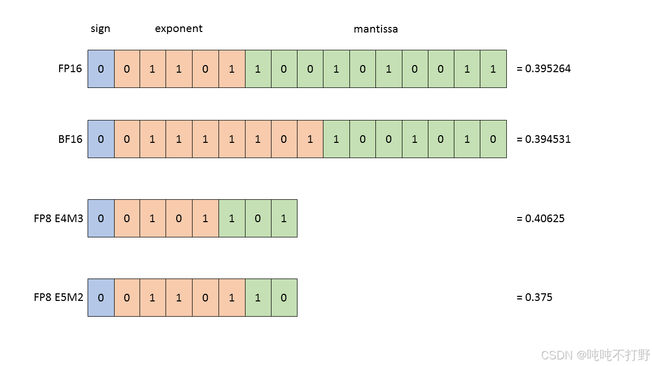
mantissa表示尾数,定点部分,小数部分
The FP8 datatype supported by H100 is actually 2 distinct datatypes, useful in different parts of the training of neural networks:
- E4M3 - it consists of 1 sign bit, 4 E xponent bits and 3 bits of M antissa. It can store values up to
+/-448and nan. - E5M2 - it consists of 1 sign bit, 5 exponent bits and 2 bits of M antissa. It can store values up to
+/-57344, +/- inf and nan. The tradeoff of the increased dynamic range is lower precision of the stored values.
选择哪种FP8类型,取决于你是想要更大的动态范围(dynamic range, 选FP8 E5M2),还是想要更高的分辨率(resolution, 选FP8 E4M3)
另外,从H100才开始支持FP8数据类型的,Using FP8 and FP4 with Transformer Engine,其他的GPU是否支持需要看详细情况
关于使用FP8进行训练的效果,详见论文:FP8 Formats for Deep Learning,这里放张图
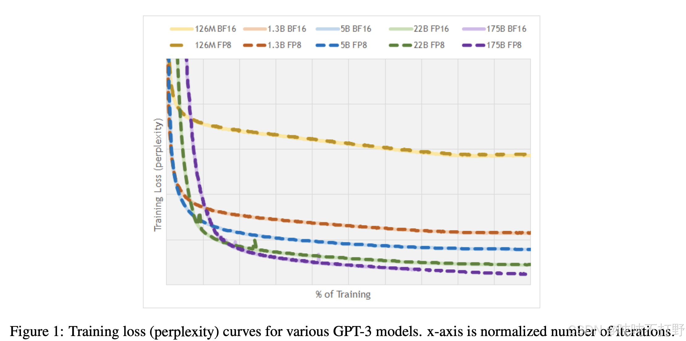
对训练的影响:
- 使用FP32训练,非常安全,就是比较耗内存
- 使用FP8或者FP16,甚至是BF16,都是有一定风险的,可能会导致训练不稳定。
- 一般来说,不会在深度学习中用FP16来训练模型。
- 同时,可以查看训练的pipeline中的任意阶段中的任意数值,前向或反向,优化器状态或者梯度累积,来确定哪些参数在哪些特定环节需要的最小精度(minimum precision)是多少。
- 这就涉及到了混合精度训练
- 解决方案:使用混合精度训练(mixed precision training ), 例如:
- 对Attention部分使用FP32
- 对涉及矩阵乘法的简单前向传播,使用BF16
关于混合精度训练:
- 数据类型选择的权衡: FP32,FP16,BF16
- Higher precision: more accurate/stable, more memory, more compute
- Lower precision: less accurate/stable, less memory, less compute
- 如何两全其美?
- use float32 by default, but use {bfloat16, fp8} when possible.
- 例如:
- Use {bfloat16, fp8} for the forward pass (activations).
- Use float32 for the rest (parameters, gradients).
- 论文:Mixed Precision Training
- Pytorch有一个自动混合精度库(
automatic mixed precision (AMP)) - NVIDIA 的 Transformer Engine 支持在线性层中使用 FP8。
- 在整个训练过程中广泛使用 FP8。FP8-LM: Training FP8 Large Language Models
3. Compute accounting
3.1 tensors_on_gpus()
默认情况下,Tensor是存储在CPU的
python
import torch
x = torch.zeros(32, 32)
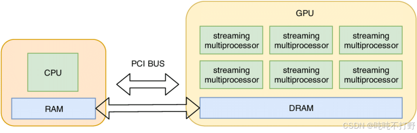
assert x.device == torch.device("cpu")CPU计算会比GPU慢很多,为了充分利用GPU的并行计算能力,一般会把数据/Tensor从CPU移动到GPU中(下图只是个示意图,从CPU到GPU的传输过程会有一些cost)
python
import torch

if not torch.cuda.is_available():
	return
num_gpus = torch.cuda.device_count()
print(num_gpus)  # 1

for i in range(num_gpus):
    properties = torch.cuda.get_device_properties(i)
    print(properties)
# "_CudaDeviceProperties (name= 'NVIDIA H100 80GB HBM3', major=9, minor=0, total_memory=81090M,
# multi_processor_count=132, uuid=11le219ad-188d-739-bf14-e59e9c1f25d2, L2_cache_size=50MB)"

memory_allocated = torch.cuda.memory_allocated()
print(memory_allocated)  # 0   这里x是在cpu的,所以gpu还没有分配

# 1. Move the tensor to GPU memory (device 0)
x = torch.zeros(32, 32)
y = x.to("cuda:0")
assert y.device == torch.device("cuda", 0)

# 2. create a tensor directly on the GPU
z = torch.zeros(32, 32, device="cuda:0")
new_memory_allocated = torch.cuda.memory_allocated()
# 这里应该有y和z两个 32*32的默认float32的浮点数矩阵
print(new_memory_allocated)  # 8192    32*32*2*4


memory_used = new_memory_allocated - memory_allocated
print(memory_used) # 8192
assert memory_used == 2 * (32 * 32 * 4)
3.2 tensor_operations()
深度学习中,大部分的tensor都是通过操作其他tensors得到的,比如:一般会读取图像或者文本作为初始tensors,之后不管是训练或者推理,中间的激活值以及输出的结果都是通过输入的tensor进行操作得到的。
3.2.1 tensor_storage()
Tensor是一种数学对象,在pytorch中,tensors对应的其实是指向已分配内存的指针(C++)
PyTorch tensors are pointers into allocated memory with metadata describing how to get to any element of the tensor. PyTorch docs
如果对opencv很了解的话,tensor和opencv的mat其实很像,本质都是指针,然后包含一些帮助确定数据在内存中存储范围/形式的元数据
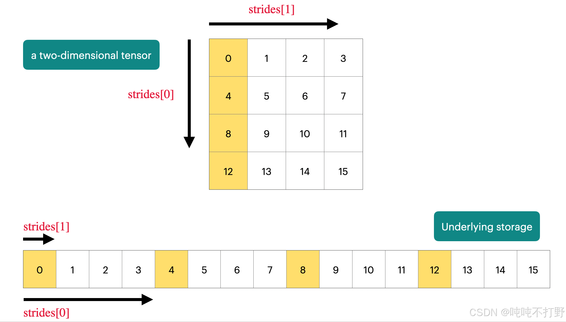
图自:Demystifying Pytorch's Strides Format
上图表示,
- 对于一个二维的 4 × 4 4\times 4 4×4的tensor,其在内存中实际存储的形式其实是一个长数组的形式(一串连续的内存单元)
- 每个维度上都会有一个strides,
- 维度0/行维度上,每次的步长是列数,即4,即每次换一行需要走4步;
- 维度1/列维度上,每次步长是1,即每次换一列需要走一步。
- 这部分更具体的内容可以看看opencv的mat类型:学习Opencv(蝴蝶书/C++)------4.图形和大型数组类型(上)中的2 存储方式,存储位置计算
python
import torch
x = torch.tensor([
        [0., 1, 2, 3],
        [4, 5, 6, 7],
        [8, 9, 10, 11],
        [12, 13, 14, 15],
    ])
# To go to the next row (dim 0), skip 4 elements in storage.
assert x.stride(0) == 4
# To go to the next column (dim 1), skip 1 element in storage.
assert x.stride(1) == 1

print(x.stride(0), x.stride(1))  # 4  1

# To find an element,这里比如要索引row=1,col=2的元素
r, c = 1, 2
# print(x[1,2])  # tensor(6.)
index = r * x.stride(0) + c * x.stride(1)
assert index == 6
# index 6 对应的值刚好就是6 这里举的例子刚好值就等于一维的索引值,即相对于tensor第一个值(指针的首地址)的偏移值
3.2.2 tensor_slicing()
这种通过指针(存储首地址)+偏移等元数据,来表示tensor(opencv的mat)的方案,可以很好的共享内存,不需要经常复制数据。
- 比如:一个tensor,需要用到其中的某一部分,而不是所有的数据,就可以只修改数据偏移(元数据)等信息,而不需要重新申请内存,完全创建一个新的变量
- 如果存在共享内存的情况,就需要很好的分清楚深拷贝和浅拷贝,以及对这个变量的修改会不会影响到原始变量的问题。
Many operations simply provide a different view of the tensor. This does not make a copy, and therefore mutations in one tensor affects the other.
像切片, reshape这类操作,本质是tensor的另一个view,torch.Tensor.view
python
import torch
def same_storage(x: torch.Tensor, y: torch.Tensor):
    return x.untyped_storage().data_ptr() == y.untyped_storage().data_ptr()

# 浅拷贝,只是创建了x的另一个view而已 共享内存

x = torch.tensor([[1., 2, 3], [4, 5, 6]])
# 1. Get row 0
y = x[0]
assert torch.equal(y, torch.tensor([1., 2, 3]))
assert same_storage(x, y)
print(id(x)) # 140199955344976, 注意,这个x是torch类型,不是python原生类型,所以返回的不是内存地址
print(id(y)) # 140199955129344
print(x.untyped_storage().data_ptr()) # 140199860077504
print(y.untyped_storage().data_ptr()) # 140199860077504

# 2. Get column 1:
y = x[:, 1]
assert torch.equal(y, torch.tensor([2, 5]))
assert same_storage(x, y)

# 3. View 2x3 matrix as 3x2 matrix:
y = x.view(3, 2)
assert torch.equal(y, torch.tensor([[1, 2], [3, 4], [5, 6]]))
assert same_storage(x, y)

# 4. Transpose the matrix:
y = x.transpose(1, 0)
assert torch.equal(y, torch.tensor([[1, 4], [2, 5], [3, 6]]))
assert same_storage(x, y)

# 5. Check that mutating x also mutates(遗传改变,基因突变) y.
x[0][0] = 100
assert y[0][0] == 100
和opencv一样,这种依靠地址索引数组的方式,会对连续性有要求,opencv的很多操作也需要在进行前保证连续性,
Note that some views are non-contiguous entries, which means that further views aren't possible.
python
import torch
x = torch.tensor([[1., 2, 3], [4, 5, 6]])
y = x.transpose(1, 0)
assert not y.is_contiguous() # 转置后, y本身是不连续的,即:y的内存索引是不连续的,但是不影响x的内存索引是连续的
try:
    y.view(2, 3)
    assert False
except RuntimeError as e:
    assert "view size is not compatible with input tensor's size and stride" in str(e)
# 这段代码没有输出东西,所以可以理解为在执行 y.view时就进入了except,同时报错信息中包含上面这段信息

# 如果直接执行view,就会报错
In [4]: y.view(2, 3)
---------------------------------------------------------------------------
RuntimeError                              Traceback (most recent call last)
Cell In[4], line 1
----> 1 y.view(2, 3)

RuntimeError: view size is not compatible with input tensor's size and stride (at least one dimension spans across two contiguous subspaces). Use .reshape(...) instead.

# 因此,可以在执行操作前强制变成连续,One can enforce a tensor to be contiguous first:
# 类似opencv的 mat.isContinuous(),然后执行clone或者copyTo()进行深拷贝,其实就是新申请一片连续的内存地址放进去。
y = x.transpose(1, 0).contiguous().view(2, 3)
assert not same_storage(x, y)Views are free, copying take both (additional) memory and compute.
单纯的slice(切片)或者dicing(切丁,切块)都属于创建一个view的操作,不会分配内存,是免费的;而copying操作是需要额外的内存的。
- Returns a tensor with the same data and number of elements as
input, but with the specified shape. - When possible, the returned tensor will be a view of
input. 此时torch.reshape=torch.view - Otherwise, it will be a copy. 此时
torch.reshape = torch.view.contiguous - Contiguous inputs and inputs with compatible strides can be reshaped without copying, but you should not depend on the copying vs. viewing behavior.
3.2.3 tensor_elementwise()
These operations apply some operation to each element of the tensor and return a (new) tensor of the same shape.
这类型的逐元素操作,会对原始的张量的所有数据发生改变,此时默认就会重新分配内存,创建一个崭新的张量了.
python
import torch
x = torch.tensor([1, 4, 9])
assert torch.equal(x.pow(2), torch.tensor([1, 16, 81]))
print(x.pow(2).untyped_storage().data_ptr(), x.untyped_storage().data_ptr())
# 140640886639872 140640888799232
assert torch.equal(x.sqrt(), torch.tensor([1, 2, 3]))
assert torch.equal(x.rsqrt(), torch.tensor([1, 1 / 2, 1 / 3]))  # i -> 1/sqrt(x_i)
assert torch.equal(x + x, torch.tensor([2, 8, 18]))
assert torch.equal(x * 2, torch.tensor([2, 8, 18]))
assert torch.equal(x / 0.5, torch.tensor([2, 8, 18]))
有一种操作在创建掩码的时候很有用
python
# triu() takes the upper triangular part of a matrix.
x = torch.ones(3, 3).triu()
assert torch.equal(x, torch.tensor([
   [1, 1, 1],
   [0, 1, 1],
   [0, 0, 1]],
))
This is useful for computing an causal attention mask, where M[i, j] is the contribution of i to j.torch.triu,这个函数在计算causal注意力掩码(M[i,j]表示i 对j的贡献,此时,需要M[i,j]是个上三角矩阵------主对角线以下都是零的方阵称为上三角矩阵)时,很重要。
3.2.4 tensor_matmul()
深度学习的核心操作就是矩阵乘法,GEMM(GeneralMatrixto Matrix Multiplication,通用矩阵的矩阵乘法)优化就足够说明这个操作的重要性了。
python
import torch

x = torch.ones(16, 32)
w = torch.ones(32, 2)
y = x @ w   # 是矩阵乘法,等同于tensor.matmul(), 不是 x*w(torch.mul(x,w))
assert y.size() == torch.Size([16, 2])
对于NLP领域的深度学习算法,在训练的时候,数据被组织的维度一般是:批次(batch),序列(sequence),然后是你想处理的东西,如下图所示:

In general, we perform operations for every example in a batch and token in a sequence.
python
import torch
# 这例子就是:
# 有4个batch,每个batch有8个样本,每个样本(sequence)有16个token,每个sequence长度是32维
x = torch.ones(4, 8, 16, 32)
w = torch.ones(32, 2)
y = x @ w
# 经过这个操作,相当于把16个token从32维压缩/降到了2维
assert y.size() == torch.Size([4, 8, 16, 2])
3.3 tensor_einops()
本质上是一种更具有可读性的写法,主要是以后看一些库的源码的时候得认识,不是非要自己也按照这个去写~
3.3.1 使用einops的motivation
传统的pytorch代码
python
import torch
x = torch.ones(2, 2, 3)  # batch, sequence, hidden
y = torch.ones(2, 2, 3)  # batch, sequence, hidden
z = x @ y.transpose(-2, -1)  # batch, sequence, sequence

# torch.transpose(input, dim0, dim1) → Tensor
# Returns a tensor that is a transposed version of input. The given dimensions dim0 and dim1 are swapped.
#In [2]: y.transpose(-2, -1).shape
#Out[2]: torch.Size([2, 3, 2])当要操作的维度比较多时,就会很容易搞混,尤其是维度的索引有反向索引(-2,-1这样的倒着的索引),而einops库可以对每个维度起名字,这样就不容易搞混了,这就是引入einops库的动机。
3.3.2 jaxtyping类型注释
此外,还有一个JAXTyping的库,是用来在types中指定dimension,但是这个库主要是用来进行typing(即:辅助静态检查),无法直接使用这个库来通过对维度的名称进行索引,还需要einops才行。
python
import torch
# Old way:
x = torch.ones(2, 2, 1, 3)  # batch seq heads hidden

# New (jaxtyping) way:
# pip install jaxtyping
from jaxtyping import Float
import torch
x: Float[torch.Tensor, "batch seq heads hidden"] = torch.ones(2, 2, 1, 3)

# 类型注解语法(Type Annotation)Python 3.5+ 支持在变量声明时添加类型提示,语法为:
variable: Type = value
# 这不会影响运行时行为(Python 仍是动态类型),但有助于代码可读性、IDE 提示和静态类型检查工具

Float[TensorType, "dim1 dim2 ..."]
# 这个语法就来自jaxtyping的结合
将代码写成这种形式,则就算是调试,也可以清晰的看到这个张量的结构和每个维度的意义,比注释要便利很多~
关于jaxtyping,
- 不是google的jax的jax.typing module,而是kidger的jaxtyping
- 前身是torchtyping,torchtyping库的目的就是:
Type annotations for a tensor's shape, dtype, names:
python
# 原始的torch写法
def batch_outer_product(x: torch.Tensor, y: torch.Tensor) -> torch.Tensor:
    # x has shape (batch, x_channels)
    # y has shape (batch, y_channels)
    # return has shape (batch, x_channels, y_channels)

    return x.unsqueeze(-1) * y.unsqueeze(-2)

# 用torchtyping可以将上述写法改为:
def batch_outer_product(x:   TensorType["batch", "x_channels"],
                        y:   TensorType["batch", "y_channels"]
                        ) -> TensorType["batch", "x_channels", "y_channels"]:

    return x.unsqueeze(-1) * y.unsqueeze(-2)
# 即:在以前的类型描述中添加了张量的shape,以及每个维度的名称描述

# jaxtyping的写法
from jaxtyping import Array, Float, PyTree

# Accepts floating-point 2D arrays with matching axes
# You can replace `Array` with `torch.Tensor` etc.
def matrix_multiply(x: Float[Array, "dim1 dim2"],
                    y: Float[Array, "dim2 dim3"]
                  ) -> Float[Array, "dim1 dim3"]:
    ...

# jaxtyping最常用的语法就是:https://docs.kidger.site/jaxtyping/api/array/
# The shape and dtypes of arrays can be annotated in the form dtype[array, shape], such as Float[Array, "batch channels"].
3.3.3 einops使用
einops是个python库,需要额外安装,Github-arogozhnikov/einops。这个库的关键介绍:
- 灵活而强大的张量操作,助您编写清晰可靠的代码(支持 PyTorch、JAX、TensorFlow 等)
- Flexible and powerful tensor operations for readable and reliable code (for pytorch, jax, TF and others)
- ✅einops教程
- Einops 是一个用于操作张量的库,会给张量的每个维度显示命名一个名称。是受到爱因斯坦求和记号(Einstein, 1916)的启发。
- Einops is a library for manipulating tensors where dimensions are named.
- It is inspired by Einstein summation notation (Einstein, 1916).
3.3.3.1 einops的einsum和torch.einsum
python
# pip install einops
from einops import rearrange, einsum, reduce
from jaxtyping import Float
# 不再使用索引的数字来表示维度,而是直接对每个维度起个名字,基于名字进行索引

# Einsum 是一种具有良好维度管理的广义矩阵乘法。
# Define two tensors:
x: Float[torch.Tensor, "batch seq1 hidden"] = torch.ones(2, 3, 4)
y: Float[torch.Tensor, "batch seq2 hidden"] = torch.ones(2, 3, 4)

# Old way:
z = x @ y.transpose(-2, -1)  # batch, sequence, sequence

# New (einops) way:
z = einsum(x, y, "batch seq1 hidden, batch seq2 hidden -> batch seq1 seq2")
# 语法就是写下x和y各自所有的维度名称,然后 ->, 然后写结果中应该出现的维度名称
# Dimensions that are not named in the output are summed over.
# 所有输出中没有出现的命名维度,都会被求和;所有输出中出现的命名维度,都会被遍历

# Or can use ... to represent broadcasting over any number of dimensions:
# 也可以用...表示剩下的所有维度
# 使用逗号区分不同的张量维度
z = einsum(x, y, "... seq1 hidden, ... seq2 hidden -> ... seq1 seq2") 关于einsum为什么可以自动完成 维度交换和矩阵乘法两种操作,详见:
-
python
# batch matrix multiplication
As = torch.randn(3, 2, 5)
Bs = torch.randn(3, 5, 4)
torch.einsum('bij,bjk->bik', As, Bs)
关键内容:
- einsum函数就是根据上面的标记法实现的一种函数,可以根据给定的表达式进行运算,可以替代但不限于以下函数:
- 矩阵求迹:trace
- 求矩阵对角线:diag
- 张量(沿轴)求和:sum
- 张量转置:transopose
- 矩阵乘法:dot
- 张量乘法:tensordot
- 向量内积:inner
- 外积:outer
3.3.3.2 einops的reduce
You can reduce a single tensor via some operation (e.g., sum, mean, max, min).
reduce只作用于一个tensor,会对一个tensor的一个或者多个维度进行聚合(aggregates)。关于reduce,也经常会在分布式系统中看到,比如:分布式训练中All-Reduce、All-Gather、Reduce-Scatter原理介绍
python
from einops import rearrange, einsum, reduce
from jaxtyping import Float
import torch
x: Float[torch.Tensor, "batch seq hidden"] = torch.ones(2, 3, 4)

# Old way
y = x.mean(dim=-1)

# New (einops) way
y = reduce(x, "... hidden -> ...", "sum")
# 左侧有hidden,右侧结果中没有hidden,说明hidden这个维度消失了,即聚合操作在hidden维度上进行

In [8]: reduce(x,"... hidden->...","sum")
Out[8]:
tensor([[4., 4., 4.],
        [4., 4., 4.]])
# 注意,三个点后面有个空格,然后再hidden,不然会报错
# EinopsError:  Error while processing sum-reduction pattern "...hidden->...".
# Input tensor shape: torch.Size([2, 3, 4]). Additional info: {}.
# Invalid axis identifier: ...hidden
# not a valid python identifier关于einops.reduce函数,
bash
reduce(
tensor: Union[~Tensor, List[~Tensor]],
pattern: str,
reduction: Union[str, Callable[[~Tensor, Tuple[int, ...]], ~Tensor]], **axes_lengths: Any) -> ~Tensor

reduction: one of available reductions ('min', 'max', 'sum', 'mean', 'prod', 'any', 'all').
Alternatively, a callable f(tensor, reduced_axes) -> tensor can be provided.
# 'prod' 的含义是:计算所有元素的乘积(product)。
# reduction操作,在pytorch的一些损失函数中也有,例如:
# https://docs.pytorch.org/docs/stable/generated/torch.nn.CrossEntropyLoss.html
3.3.3.3 einops的rearrange
Sometimes, a dimension represents two dimensions and you want to operate on one of them.
有时候一个dim可能代表多个dims,需要先解压缩unpack,然后操作其中的某个dim,然后再pack压缩回一个dim中。
python
from einops import rearrange, einsum, reduce
from jaxtyping import Float
import torch
x: Float[torch.Tensor, "batch seq total_hidden"] = torch.ones(2, 3, 8)
# where total_hidden is a flattened representation of heads * hidden1
w: Float[torch.Tensor, "hidden1 hidden2"] = torch.ones(4, 4)

# Break up total_hidden into two dimensions (heads and hidden1):
x = rearrange(x, "... (heads hidden1) -> ... heads hidden1", heads=2)
# Perform the transformation by w:
x = einsum(x, w, "... hidden1, hidden1 hidden2 -> ... hidden2")
# Combine heads and hidden2 back together:
x = rearrange(x, "... heads hidden2 -> ... (heads hidden2)")

# 所以rearrange的作用就是解压缩一个维度到多个维度;或者reshape/view压缩多个维度到一个维度,flatten
einops.rearrangeis a reader-friendly smart element reordering for multidimensional tensors.- This operation includes functionality of
transpose (axes permutation),reshape (view),squeeze,unsqueeze,stack,concatenateand other operations.
3.4 tensor_operations_flops()
3.4.1 基本介绍( FLOPs vs. FLOP/s vs FLOPS)
关于张量操作的成本(tensor operation cost),上面介绍了很多关于张量的操作,这里关注下这些操作的成本~
A floating-point operation (FLOP) is a basic operation like addition (x + y) or multiplication (x y).
关于基础操作,可以看看: 本文中X. 1. 加减乘除都是用加法器实现的? 的部分
术语的发音混淆(pronounced the same!):
- FLOPs: floating-point operations (measure of computation done)
- 浮点数操作的次数,衡量完成的计算量
- FLOP/s: floating-point operations per second (also written as
FLOPS), which is used to measure the speed of hardware.- GPU每秒钟可以进行的浮点数运算次数,用来衡量硬件的计算速度。
- 本课程里统一使用
FLOP/s来表示每秒钟的浮点数运算次数,不用FLOPS表示,容易搞混。
3.4.2 直观感受
常见的一些LLM训练所使用的(总)浮点数运算次数(FLOPs):
- Training GPT-3 (2020) took 3.14e23 FLOPs. article
- GPT-3 175B model required
3.14E23FLOPS of computing for training. Even at theoretical 28 TFLOPS for V100 and lowest 3 year reserved cloud pricing we could find, this will take 355 GPU-years and cost $4.6M for a single training run. Similarly, a single RTX 8000, assuming 15 TFLOPS, would take 665 years to run.
- GPT-3 175B model required
- Training GPT-4 (2023) is speculated to take 2e25 FLOPs(推测~) article
- It took about 2 × 10 25 2 \times 10^{25} 2×1025 FLOPS to train, with 13 trillion token (passes).
- US executive order: any foundation model trained with >= 1e26 FLOPs must be reported to the government (revoked in 2025)
- 美国行政命令:任何使用不少于 1e26 次浮点运算(FLOPs)训练的基础模型都必须向政府申报(该命令已于 2025 年撤销)。
- 欧盟的人工智能法案是1e25,而且还没撤销
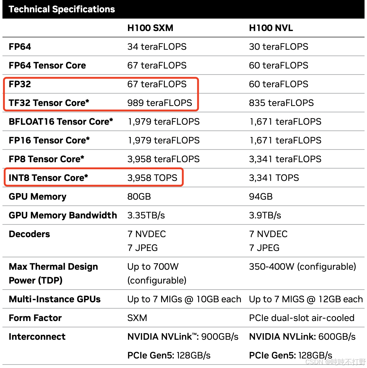
- A100 has a peak performance of 312 teraFLOP/s spec, teraFLOP/s是每秒 10 12 10^{12} 1012次浮点数运算
- H100 has a peak performance of 1979 teraFLOP/s with sparsity, 50% without spec,
- 如果老师课程里的链接打不开,我这里放了更新过的
- 想要去搜某个特定型号显卡的DataSheet,直接搜索
nvidia-tensor-core-gpu-datasheet h100这样的关键字就好了 - https://resources.nvidia.com/en-us-tensor-core/nvidia-tensor-core-gpu-datasheet这个链接已经失效了,但是应该以前是用来链接到最新的显卡的,所以关键词就是
nvidia-tensor-core-gpu-datasheet
python
  # 8 H100s for 2 weeks:
 h100_flop_per_sec == 1979e12 / 2
 total_flops = 8 * (60 * 60 * 24 * 7) * h100_flop_per_sec
 # total_flops=4.788e+21
 # GPT3是3.14E23的浮点数运算,也就是还差两个数量级,就是需要100个上面的运算量
下图可以知道,通常我们说一个GPU的FLOP/s,一般指的是 BF16的运算次数,如果不是BF16,而是更高精度的FP32,则FLOP/s则会更低。
另外,下图的*号,表示带有稀疏性,但是大模型里很多操作都是稠密的,所以实际的BF16的FLOP/s还要再减小一半。
3.4.3 以线性模型为例计算矩阵乘法的运算量
这门课程不会讲transformer,所以如果想要看transformer的计算量,需要自己分析。
以简单的线性模型为例,就足够去理解运算量的计算了~
线性模型的基本描述:
- 有 n n n个点, 即数据集大小/样本数为 n n n
- 每个点都是 d d d维
- 线性模型的作用是: 将每个 d d d维向量映射成一个 k k k维向量
python
import torch

def get_device(index: int = 0) -> torch.device:
    """Try to use the GPU if possible, otherwise, use CPU."""
    if torch.cuda.is_available():
        return torch.device(f"cuda:{index}")
    else:
        return torch.device("cpu")

if torch.cuda.is_available():
      B = 16384  # Number of points
      D = 32768  # Dimension
      K = 8192   # Number of outputs
  else:
      B = 1024
      D = 256
      K = 64
device = get_device()
x = torch.ones(B, D, device=device)
w = torch.randn(D, K, device=device)
y = x @ w
上面这个代码没有用梯度下降,反向传播求导来优化 w w w权重矩阵,只是单纯给一个计算示例。
注意,这里老师讲的有问题,用Qwen3-Max/chatGPT问问就知道了,我下面给的是正确答案~
y = x @ w y=x@w y=x@w这个矩阵乘法公式的计算量是多少?
- 参考✅一个函数打天下,einsum,
- c i j = a i j b j k = ∑ j a i j b j k c_{ij} = a_{ij}b_{jk}=\sum_{j}a_{ij}b_{jk} cij=aijbjk=∑jaijbjk
- 用爱因斯坦求和标记来表示上面这个乘法就是:
- y b k = x b d w d k = ∑ d x b d w d k = ∑ d = 1 D x b d w d k y_{bk}=x_{bd}w_{dk}=\sum_{d}x_{bd}w_{dk}=\sum_{d=1}^{D}x_{bd}w_{dk} ybk=xbdwdk=∑dxbdwdk=∑d=1Dxbdwdk
- 对于输出的 y y y, 一共有 B × K B\times K B×K个元素, 即: B B B个输出,每个输出是 K K K维度;
- 对于 y y y中的每个元素,都是进行过D次乘法,即有 D D D组 x b d w d k x_{bd}w_{dk} xbdwdk,这 D D D组 x b d w d k x_{bd}w_{dk} xbdwdk还需要进行 D − 1 D-1 D−1次加法,来求和
- 所以总的运算次数是: B × K × ( D + D − 1 ) = B × K × 2 D − B × K B\times K \times (D+D-1)=B\times K \times 2D-B\times K B×K×(D+D−1)=B×K×2D−B×K
- 矩阵乘法的时间复杂度为: O ( B D K ) O(_{BDK}) O(BDK)
- 标准算法的浮点运算总数(FLOPs)通常定义为 乘法 + 加法:
- FLOPs= B × K × 2 D − B × K = 2 B D K − B K B\times K \times 2D-B\times K=2BDK-BK B×K×2D−B×K=2BDK−BK
- 通常近似为 2 B D K 2BDK 2BDK(尤其当 D D D 较大时)
- 在CS231n课程靠后的内容里,韩松老师好像在讲硬件和运算效率的时候说过这部分~
结论
矩阵乘法的运算量,通常是两个矩阵的三个不同维度的乘积的2倍,即:
x = torch.ones(B, D)
w = torch.randn(D, K)
y = x @ w
计算y所需要的运算量是: 2BDK
即:矩阵乘法的运算量,和矩阵维度是线性正相关的
3.4.4 其他矩阵操作的运算量
- 单个 m × n m\times n m×n的矩阵,进行逐元素操作(Elementwise operation )的计算量就是 O ( m n ) O(mn) O(mn)
- 两个 m × n m\times n m×n的矩阵进行加法,计算量就是 m × n m\times n m×n次加法
- 在深度学习中涉及的矩阵运算里,没有比矩阵乘法更expensive的操作了
- 因此,很多时候计算运算量,会忽略那些计算量小的操作,而只关注矩阵乘法~
- 如果矩阵比较小,那么其他操作就不能忽略了,但是在transformer模型里,没有很小的矩阵。。。同时,硬件的很多优化都是针对矩阵乘法进行的。
3.4.5 推广到transformers的计算量
对于线性模型中举例的矩阵乘法运算量,可以理解为:
- B is the number of data points(B是数据量)
- (D K) is the number of parameters(DK是参数量)
- FLOPs for forward pass is 2 (# tokens) (# parameters)
- #表示 xxx的数量,上面这个计算可以表示为: 2 × t o k e n s × p a r a m e t e r s 2\times tokens \times parameters 2×tokens×parameters
- 即:单次前向计算的浮点数运算次数为: 2 × t o k e n s × p a r a m e t e r s 2\times tokens \times parameters 2×tokens×parameters,这里的
tokens也可以是number of data points
- It turns out this generalizes to Transformers (to a first-order approximation).
这部分计算仅仅是一个近似,在CS336------1. Overview的2.2.2 小语言模型和LLM的区别部分中,放过一张图,随着模型参数量增加,transformers模型中不同组件/层消耗的FLOPS差异
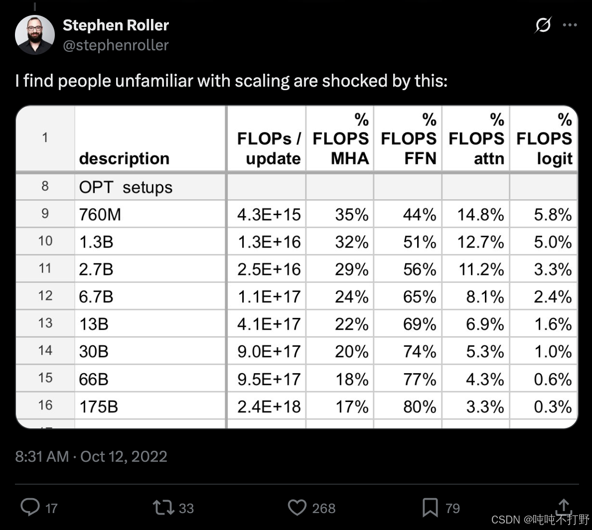
-
FFN使用的就是MLP,即多层感知机,就是多个线性层拼起来最朴实的那种网络
-
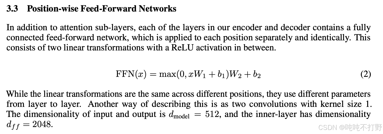
大致看一下transformer中ffn组件的实现:
python# https://github.com/pytorch/pytorch/blob/v2.9.1/torch/nn/modules/transformer.py#L645 # TransformerEncoderLayer is made up of self-attn and feedforward network. # 先找 class TransformerEncoderLayer # https://github.com/pytorch/pytorch/blob/v2.9.1/torch/nn/modules/transformer.py#L751 # 再就是 # Implementation of Feedforward model self.linear1 = Linear(d_model, dim_feedforward, bias=bias, **factory_kwargs) self.dropout = Dropout(dropout) self.linear2 = Linear(dim_feedforward, d_model, bias=bias, **factory_kwargs) # 就是一个两层的MLP -
再看一眼论文里的原始描述:Attention Is All You Need
3.4.6 理论计算速度和实际计算速度
How do our FLOPs calculations translate to wall-clock time (seconds)?
- wall-clock time 挂钟时间:指实际经过的时间,与计算机程序中的CPU时间不同,它包括了程序执行过程中的等待时间和其他外部因素的影响。
python
import torch
def time_matmul(a: torch.Tensor, b: torch.Tensor) -> float:
    """Return the number of seconds required to perform `a @ b`."""
    # Wait until previous CUDA threads are done
    if torch.cuda.is_available():
        torch.cuda.synchronize()
    def run():
        # Perform the operation
        a @ b
        # Wait until CUDA threads are done
        if torch.cuda.is_available():
            torch.cuda.synchronize()
    # Time the operation `num_trials` times
    num_trials = 5
    total_time = timeit.timeit(run, number=num_trials)
    return total_time / num_trials

device = ""
if torch.cuda.is_available():
	B = 16384  # Number of points
    D = 32768  # Dimension
    K = 8192   # Number of outputs
    device = torch.device(f"cuda:{index}")
else:
    B = 1024
    D = 256
    K = 64
    device = torch.device("cpu")
x = torch.ones(B, D, device=device)  # 这里默认是torch.float32的精度
w = torch.randn(D, K, device=device)
actual_time = time_matmul(x, w)
actual_flop_per_sec = actual_num_flops / actual_time
# 下面结果是在H100上进行的
# total_flops = 4.788e+21
# actual_num_flops = 8.796e+12
# actual_time = 0. 163
# actual_flop_per_sec = 5.407e+13

# 和显卡标称的FLOP/s相比
def get_promised_flop_per_sec(device: str, dtype: torch.dtype) -> float:
    """Return the peak FLOP/s for `device` operating on `dtype`."""
    if not torch.cuda.is_available():
        No CUDA device available, so can't get FLOP/s.
        return 1
    properties = torch.cuda.get_device_properties(device)
    if "A100" in properties.name:
        # https://www.nvidia.com/content/dam/en-zz/Solutions/Data-Center/a100/pdf/nvidia-a100-datasheet-us-nvidia-1758950-r4-web.pdf")
        if dtype == torch.float32:
            return 19.5e12
        if dtype in (torch.bfloat16, torch.float16):
            return 312e12
        raise ValueError(f"Unknown dtype: {dtype}")
    if "H100" in properties.name:
        # https://resources.nvidia.com/en-us-tensor-core/nvidia-tensor-core-gpu-datasheet")
        if dtype == torch.float32:
            return 67.5e12
        if dtype in (torch.bfloat16, torch.float16):
            return 1979e12 / 2  # 1979 is for sparse, dense is half of that
        raise ValueError(f"Unknown dtype: {dtype}")
    raise ValueError(f"Unknown device: {device}")

promised_flop_per_sec = get_promised_flop_per_sec(device, x.dtype)

# actual_flop_per_sec = 5.407e+13   # 实际运算的FLOP/s是  5.407e+13
# promised_flop_per_sec = 6.750e+13  # H100标称的FLOP/s是 6.750e+13
# In [1]: (6.75-5.407)/6.75
# Out[1]: 0.19896296296296295
# 损失了差不多20%的性能

# 如果是BF16,则
x = x.to(torch.bfloat16)
w = w.to(torch.bfloat16)
bf16_actual_time = time_matmul(x, w)
bf16_actual_flop_per_sec = actual_num_flops / bf16_actual_time
bf16_promised_flop_per_sec = get_promised_flop_per_sec(device, x.dtype)
bf16_mfu = bf16_actual_flop_per_sec / bf16_promised_flop_per_sec
# bf16_actual_time = 0.032
# bf16_actual_flop_per_sec = 2.735e+14
# bf16_promised_flop_per_sec = 9.895e+14
# bf16_mfu = 0.276

# float32位
# total_flops = 4.788e+21
# actual_num_flops = 8.796e+12
# actual_time = 0. 163
# actual_flop_per_sec = 5.407e+13
# f32_mfu=0.801
显卡标称的FLOP/s:
上述Float32和bf16的结果可以看出:
-
bf16的计算速度要更高,同样的矩阵乘法,bf16是0.032s,float32是0. 163, 5倍
bashIn [3]: 0.163/0.032 Out[3]: 5.09375 -
actual_flop_per_sec差的则更多,
bashIn [4]: 2.735e+14/8.796e+12 Out[4]: 31.09367894497499 -
在mfu的对比上,bf16就远远低于fp32了, 0.276<0.801 ,所以NVIDIA的H100的datasheet上给的数字可能过于乐观了~
python# H00的datasheet上给的bf16的数值是针对稀疏的,所以如果要针对稠密矩阵,得除以2 # 1979e12 / 2 # 1979 is for sparse, dense is half of that # 而给的fp32本身就不带星号,所以不是针对稀疏的,就不用除
3.4.7 MFU
MFU(Model FLOPs utilization )的定义:
实际计算的 F L O P / s 显卡标称的 F L O P / s \frac{实际计算的FLOP/s}{显卡标称的FLOP/s} 显卡标称的FLOP/s实际计算的FLOP/s
(ignore communication/overhead,通常是忽略了通信和其他各种开销的情况下)
python
# 延续上面的计算
mfu = actual_flop_per_sec / promised_flop_per_sec
# MFU=0.801 通常,MFU>=0.5就很好了,如果矩阵乘法(matmuls)是主要的计算,则MFU会更高
另外,MFU(Model FLOPs utilization)的名称里更多提到的是模型相关的计算。
- 比如说模型如果进行了一些矩阵计算的优化,或者直接使用了之前某些计算的缓存
- 则这些计算实际上并没有发生
- 因此这里的
实际计算的FLOP/s,是指模型真正执行的计算,并不是完全从模型本身的参数推断的那种计算~
3.4.X 总结
- Matrix multiplications dominate: (2 m n p) FLOPs.
- 在大模型相关的计算中,矩阵乘法占主导,近似的一个前向计算过程中,FLOPs浮点数运算量的计算公式是: 2*tokens个数*模型参数
- FLOP/s depends on hardware (H100 >> A100) and data type (bfloat16 >> float32)
- Model FLOPs utilization (MFU): (actual FLOP/s) / (promised FLOP/s)
3.5 gradients_basics()
3.4 tensor_operations_flops() 这部分只说了浮点数运算,更多介绍的是前向计算过程中涉及到的计算量,实际上,还有很大一部分运算发生在梯度运算的时候~
3.4 tensor_operations_flops() 中线性模型的例子,只描述了单次的前向计算,这里依然以线性模型为例,说明一下反向传播中梯度的计算。
这里给的例子,假设有以下待确认参数的线性模型:
y = 0.5 ( x ∗ w − 5 ) 2 y = 0.5 (x * w - 5)^2 y=0.5(x∗w−5)2
最简单的一个前向和反向的例子就如下:
python
import torch
# 前向计算
x = torch.tensor([1., 2, 3])
w = torch.tensor([1., 1, 1], requires_grad=True)  # Want gradient
pred_y = x @ w
loss = 0.5 * (pred_y - 5).pow(2)

# 反向计算
loss.backward()
assert loss.grad is None
assert pred_y.grad is None
assert x.grad is None
assert torch.equal(w.grad, torch.tensor([1, 2, 3]))  # w的梯度就是 x
此时参数w的梯度就等于输入x,即w中第一个数值的梯度是1,第二个数值的梯度是2,第三个数值的梯度是3.
3.6 gradients_flops()
计算一下梯度的计算量(注意,虽然梯度也是一种张量,本质上这也是张量的FLOPS计算,但是这部分并没有放到 3.4 tensor_operations_flops() 中), 用的还是之前 3.4.3 以线性模型为例计算矩阵乘法的运算量 中的例子
python
import torch
def get_device(index: int = 0) -> torch.device:
    """Try to use the GPU if possible, otherwise, use CPU."""
    if torch.cuda.is_available():
        return torch.device(f"cuda:{index}")
    else:
        return torch.device("cpu")

if torch.cuda.is_available():
    B = 16384  # Number of points
    D = 32768  # Dimension
    K = 8192   # Number of outputs
else:
    B = 1024
    D = 256
    K = 64
device = get_device()
x = torch.ones(B, D, device=device)
w1 = torch.randn(D, D, device=device, requires_grad=True)
w2 = torch.randn(D, K, device=device, requires_grad=True)

# Model: x --w1--> h1 --w2--> h2 -> loss
# 前向
h1 = x @ w1
h2 = h1 @ w2
loss = h2.pow(2).mean()
# 反向
h1.retain_grad()  # For debugging
h2.retain_grad()  # For debugging
loss.backward()
对于上述这个两层的线性网络来说,
-
前向计算的运算量: num_forward_flops = (2BDD) + (2BDK)
-
反向运算的运算量:
bashx --w1--> h1 --w2--> h2 -> loss h1.grad = d loss / d h1 h2.grad = d loss / d h2 w1.grad = d loss / d w1 w2.grad = d loss / d w2 -
使用链式法则,以w2的梯度计算为例:
d ( l o s s ) d ( w 2 ) = d ( h 2. p o w ( 2 ) . m e a n ( ) ) d w 2 = d ( h 2. p o w ( 2 ) . m e a n ( ) ) d h 2 × d ( h 2 ) d ( w 2 ) = d ( h 2. p o w ( 2 ) . m e a n ( ) ) d h 2 × d ( h 1 @ w 2 ) d ( w 2 ) = h 2 g r a d × h 1 \begin{aligned} &\frac{d(loss)}{d(w_2)}=\frac{d(h2.pow(2).mean())}{dw_2}=\\ &\frac{d(h2.pow(2).mean())}{dh_2}\times\frac{d(h_2)}{d(w_2)}=\\ &\frac{d(h2.pow(2).mean())}{dh_2}\times\frac{d(h_1 @ w_2)}{d(w_2)}=h_2^{\mathrm{grad}}\times h_1 \end{aligned} d(w2)d(loss)=dw2d(h2.pow(2).mean())=dh2d(h2.pow(2).mean())×d(w2)d(h2)=dh2d(h2.pow(2).mean())×d(w2)d(h1@w2)=h2grad×h1 -
即: w 2 g r a d j , k = ∑ i h 1 i , j ⋅ h 2 g r a d i , k w_2^{\mathrm{grad}}j,k = \sum_{i} h_1i,j \cdot h_2^{\mathrm{grad}}i,k w2gradj,k=∑ih1i,j⋅h2gradi,k,
-
同时,也可以得到: h 1 g r a d i , j = ∑ k w 2 j , k ⋅ h 2 g r a d i , k h_1^{\mathrm{grad}}i,j = \sum_{k} w_2j,k \cdot h_2^{\mathrm{grad}}i,k h1gradi,j=∑kw2j,k⋅h2gradi,k
bashw2.grad[j,k] = sum_i h1[i,j] * h2.grad[i,k] # 这里的索引序号可能并不完全符合矩阵乘法计算的对应,考虑一下爱因斯坦求和记号,知道要表达的真正意义即可~ h1.grad[i,j] = sum_k w2[j,k] * h2.grad[i,k]
python
# 关于w2梯度的计算
# 每个参数的梯度的维度和参数本身的维度一致~
assert w2.grad.size() == torch.Size([D, K])
# h1的维度 = x*w1=(B,D)*(D,D)=(B,D)
assert h1.size() == torch.Size([B, D])
# h2的维度 = h1*w2=(B,D)*(D,K)=(B,K)
assert h2.grad.size() == torch.Size([B, K])
# 所以不考虑h2的梯度的计算量的情况下,假设h2已经计算好了,
# 则w2的梯度计算量是 在B维度上进行矩阵的乘法和加法,然后一共是D*K个元素需要进行这些操作,即
# 2*B*DK

# For each (i, j, k), multiply and add.
num_backward_flops += 2 * B * D * K

# 同理,关于h1梯度的计算
assert h1.grad.size() == torch.Size([B, D])
assert w2.size() == torch.Size([D, K])
assert h2.grad.size() == torch.Size([B, K])
# h1梯度是 h2*w2 相当于在K维度上进行矩阵乘法的乘法和加法,有B*D个元素需要进行这样的计算
# = 2*K*BD
# For each (i, j, k), multiply and add.
num_backward_flops += 2 * B * D * K
进一步,如果要计算w1的梯度,则就等于 h1的梯度 * X = (B,D)*(B,D) 在B维度上进行矩阵乘法的乘法和加法
- 则 w1梯度的计算量就是 2*B*D*D
- (2+2)*B*D*D,对于w1和x这个层,如果算了X的梯度,就是(2+2)*B*D*D了(但是X的梯度用不到)
- 同理,对于w2和h1这个层,运算量就是(2+2) * B* D * K
∂ L ∂ w 1 j , k ∑ i x i , j ⋅ h 1. g r a d i , k \frac{\partial L}{\partial w1j,k}\sum_i xi,j \cdot h1.gradi,k ∂w1j,k∂Li∑xi,j⋅h1.gradi,k
形状检查:
x:(B, D)h1.grad:(B, D)w1.grad:(D, D)
这是一个标准矩阵乘法:
text
w1.grad = xᵀ @ h1.gradFLOPs: 2 × B × D × D 2 \times B \times D \times D 2×B×D×D
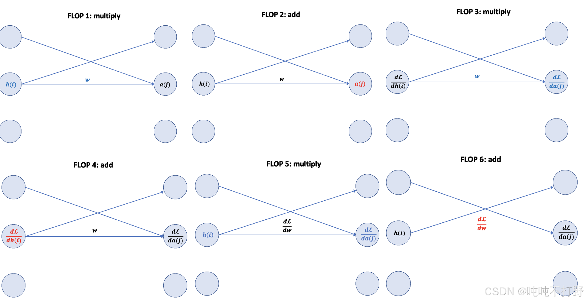
给了一个动图链接: The FLOPs Calculus of Language Model Training
这里直接拼成一个大图方便看:要稍微动点脑子,不赘述了,而且感觉怪怪的,上面链接的原文中有详细说明。
总结
对于简单的线性层,前向计算是参数量的两倍,反向计算一般是参数量的四倍(除了输入层相邻的第一个线性层之外,因为这个线性层的输入x一般不算梯度)
- Forward pass: 2 (# data points) (# parameters) FLOPs
- Backward pass: 4 (# data points) (# parameters) FLOPs
- Total: 6 (# data points) (# parameters) FLOPs
会看 1.2 引子(一些快速计算例子) 中第一个问题的 6,就是来自这里
另外,这种浮点数运算量的计算方式适合:每一步计算都涉及到一个新的参数;而不是通过参数共享只用1个参数,但是产生10亿次运算的那种。
4. Model
4.1 module_parameters()
python
import torch
from torch import nn
input_dim = 16384
output_dim = 32

# pytorch中会使用nn.Parameter这种对象来存储模型参数
# Model parameters are stored in PyTorch as nn.Parameter objects.
w = nn.Parameter(torch.randn(input_dim, output_dim))
assert isinstance(w, torch.Tensor)  # Behaves like a tensor
assert type(w.data) == torch.Tensor  # Access the underlying tensor

# 参数初始化
x = nn.Parameter(torch.randn(input_dim))
output = x @ w
assert output.size() == torch.Size([output_dim])
# 如果直接以随机方式初始化,那么在进行矩阵乘法操作后,得到的output里的值的范围就会很广泛(通常会随着input_dim增大而增大,因为会在input_dim维度上进行乘法和加法),就很容易blow up
# 此时的output
# tensor([-164.9940, -172.8086,  259.0620,   70.6158,   71.1710,  198.6639,
#       -110.6112,  154.1603,  166.4517, -108.8331, -204.5345,   51.4940,
#        -75.8735,  251.2097,   87.5925,  182.8901,  157.9116,  -54.6850,
#         8.5866,   23.6278,  233.9193,  188.6996,  -14.4043, -113.9815,
#        -51.3374,   -7.4196,    8.7242,    3.7935,  -39.3690,  -61.5695,
#        -43.3980,  158.6143], grad_fn=<SqueezeBackward4>)

# 因此,最基本的初始化就是 针对input_dim维度具有不变性 invariant to input_dim.
# 最简单的一个方案就是 rescale by 1/sqrt(input_dim)
import numpy as np
w = nn.Parameter(torch.randn(input_dim, output_dim) / np.sqrt(input_dim))
output = x @ w
# 此时的output
# tensor([ 0.7608, -0.6601,  0.3037,  0.0149,  0.1464,  0.4069,  0.1844,  0.8708,
#       -0.2195,  0.2143,  0.0576, -0.8700,  1.4222,  0.6817, -0.2631, -1.6062,
#       -2.4659,  2.6940, -1.1520, -2.4640,  1.1054,  0.5835, -0.5827, -0.2247,
#       -2.0313, -0.4954, -1.5547, -0.8008,  0.3853,  0.0155,  0.5098,  1.7307], grad_fn=<SqueezeBackward4>)

# 此时这种初始化的结果有点类似于正态分布,但是正态分布的问题在于:其尾部是无界的,会有些不安全,因此,可以直接截断避免任何异常值的可能
# To be extra safe, we truncate the normal distribution to [-3, 3] to avoid any chance of outliers.
w = nn.Parameter(nn.init.trunc_normal_(torch.empty(input_dim, output_dim), std=1 / np.sqrt(input_dim), a=-3, b=3))关于nn.Parameter
- https://docs.pytorch.org/docs/stable/generated/torch.nn.parameter.Parameter.html
- 参数(Parameters)是 Tensor 的子类,当它们与 Module 一起使用时具有一个非常特殊的属性:当它们被赋值为 Module 的属性时,会自动被添加到该模块的参数列表中,并会出现在例如 parameters() 迭代器中。而直接赋值一个普通的 Tensor 则不会产生这种效果。这是因为用户可能希望在模型中缓存一些临时状态(例如 RNN 的上一个隐藏状态)。如果没有 Parameter 这样的类,这些临时变量也会被注册为模型参数。
- 另外,如果创建了
nn.Parameter,则默认requires_grad=True, 如果只是一个普通的Tensor而没有用nn.Parameter包裹,则默认requires_grad=False - User Guide->Developer Notes->Autograd mechanics->Locally disabling gradient computation
- 自动求导-
torch.no_grad()上下文和requires_grad等的设置
- 自动求导-
- https://github.com/pytorch/pytorch/blob/main/torch/nn/parameter.py
关于好的初始化:
- Xavier initialization: Understanding the difficulty of training deep feedforward neural networks
- Is there a proper initialization technique for the weight matrices in multi-head attention?
- 详见:动手学深度学习V2.0(Pytorch)------14. 数值稳定性/模型初始化/激活函数中2.2.1 Xavier初始化 及附近内容
4.2 custom_model()
python
import torch
from torch import nn
import numpy as np

def get_device(index: int = 0) -> torch.device:
    """Try to use the GPU if possible, otherwise, use CPU."""
    if torch.cuda.is_available():
        return torch.device(f"cuda:{index}")
    else:
        return torch.device("cpu")
def get_num_parameters(model: nn.Module) -> int:
    return sum(param.numel() for param in model.parameters())

class Linear(nn.Module):
    """Simple linear layer."""
    def __init__(self, input_dim: int, output_dim: int):
        super().__init__()
        self.weight = nn.Parameter(torch.randn(input_dim, output_dim) / np.sqrt(input_dim))
    def forward(self, x: torch.Tensor) -> torch.Tensor:
        return x @ self.weight

class Cruncher(nn.Module):
    def __init__(self, dim: int, num_layers: int):
        super().__init__()
        self.layers = nn.ModuleList([
            Linear(dim, dim)
            for i in range(num_layers)
        ])
        self.final = Linear(dim, 1)
    def forward(self, x: torch.Tensor) -> torch.Tensor:
        # Apply linear layers
        B, D = x.size()
        for layer in self.layers:
            x = layer(x)
        # Apply final head
        x = self.final(x)
        assert x.size() == torch.Size([B, 1])
        # Remove the last dimension
        x = x.squeeze(-1)
        assert x.size() == torch.Size([B])
        return x

D = 64  # Dimension
num_layers = 2
model = Cruncher(dim=D, num_layers=num_layers)

param_sizes = [
        (name, param.numel())
        for name, param in model.state_dict().items()
]
assert param_sizes == [
    ("layers.0.weight", D * D),
    ("layers.1.weight", D * D),
    ("final.weight", D),
]
num_parameters = get_num_parameters(model)
assert num_parameters == (D * D) + (D * D) + D

# Remember to move the model to the GPU.
device = get_device()
model = model.to(device)
# Run the model on some data.
B = 8  # Batch size
x = torch.randn(B, D, device=device)
y = model(x)
assert y.size() == torch.Size([B])
4.3 Training loop and best practices
4.3.1 note_about_randomness
关于随机性(randomness)的一些注意事项:
- Randomness shows up in many places: parameter initialization, dropout, data ordering, etc.
- For reproducibility, we recommend you always pass in a different random seed for each use of randomness.
- Determinism is particularly useful when debugging, so you can hunt down the bug.
从最佳实践的角度考虑,为了保证最大程度的可复现性,建议在训练/相关需要设置随机数的地方,一次性进行以下三种设置:
python
# Torch
seed = 0
torch.manual_seed(seed)

# NumPy
import numpy as np
np.random.seed(seed)

# Python
import random
random.seed(seed)
4.3.2 data_loading()
In language modeling, data is a sequence of integers (output by the tokenizer).
It is convenient to serialize them as numpy arrays (done by the tokenizer).
python
import numpy as np
orig_data = np.array([1, 2, 3, 4, 5, 6, 7, 8, 9, 10], dtype=np.int32)
orig_data.tofile("data.npy")
You can load them back as numpy arrays.
Don't want to load the entire data into memory at once (LLaMA data is 2.8TB).
Use memmap to lazily load only the accessed parts into memory.
- 为了节省内存,一般不会一次性把所有数据都加载,可以使用
memmap来进行惰性加载~ - 比如:LLaMA的训练数据就有2.8TB,对于这种量级的数据,只能进行惰性加载
python
data = np.memmap("data.npy", dtype=np.int32)
assert np.array_equal(data, orig_data)
A data loader generates a batch of sequences for training.
python
import torch
def get_batch(data: np.array, batch_size: int, sequence_length: int, device: str) -> torch.Tensor:
    # Sample batch_size random positions into data.
    start_indices = torch.randint(len(data) - sequence_length, (batch_size,))
    assert start_indices.size() == torch.Size([batch_size])
    # Index into the data.
    x = torch.tensor([data[start:start + sequence_length] for start in start_indices])
    assert x.size() == torch.Size([batch_size, sequence_length])
    return x

B = 2  # Batch size
L = 4  # Length of sequence
x = get_batch(data, batch_size=B, sequence_length=L, device=get_device())
assert x.size() == torch.Size([B, L])
4.4 optimizer()
然后需要定义优化器(optimizer()),除了最经典的随机梯度下降(Stochastic Gradient descent)算法,还有一些其他的基于SGD的衍生算法:
- momentum = SGD + exponential averaging of grad
- AdaGrad = SGD + averaging by grad^2
- RMSProp = AdaGrad + exponentially averaging of grad^2
- Adam = RMSProp + momentum
4.4.1 自定义优化器+单步优化过程
python
# 回忆一下4.2 cutom_model中定义的模型
B = 2
D = 4
num_layers = 2
model = Cruncher(dim=D, num_layers=num_layers).to(get_device())

# 查看模型当前的权重,前两个层是自定义的linear层,输入和输出都是4维度,所以权重是4x4
# 最后一层是输入为4维,输出为1维,所以权重为4x1
state = model.state_dict()
# OrderedDict([('layers.0.weight',
#             tensor([[ 1.3997,  0.9533,  0.3022, -0.6394],
#                    [ 0.0286, -0.1586,  0.3253,  0.1770],
#                    [ 0.1490, -0.4214, -0.4238,  0.0264],
#                    [ 0.1031,  0.9212,  0.2085, -0.2865]])),
#            ('layers.1.weight',
#             tensor([[ 0.1753, -0.3085,  1.0922, -0.3110],
#                     [-0.8168, -0.1644,  0.0370,  0.8315],
#                     [ 0.0806, -0.0539,  1.3614, -0.0336],
#                     [ 0.7123,  0.5419,  0.2761,  0.0510]])),
#            ('final.weight',
#             tensor([[ 0.2207],
#                     [-0.9913],
#                     [ 0.6032],
#                     [-0.3366]]))])
# 造一些数据
x = torch.randn(B, D, device=get_device())
y = torch.tensor([4., 5.], device=get_device())
# 进行前向计算
pred_y = model(x)
# 得到损失函数
import torch.nn.functional as F
loss = F.mse_loss(input=pred_y, target=y)
# 基于损失函数,计算梯度
loss.backward()
# 定义一个优化器
from typing import Iterable
class AdaGrad(torch.optim.Optimizer):
    def __init__(self, params: Iterable[nn.Parameter], lr: float = 0.01):
        super(AdaGrad, self).__init__(params, dict(lr=lr))
    def step(self):
        for group in self.param_groups:
            lr = group["lr"]
            for p in group["params"]:
                # Optimizer state
                state = self.state[p]
                grad = p.grad.data
                # Get squared gradients g2 = sum_{i<t} g_i^2
                g2 = state.get("g2", torch.zeros_like(grad))
                # Update optimizer state
                g2 += torch.square(grad)
                state["g2"] = g2
                # Update parameters
                p.data -= lr * grad / torch.sqrt(g2 + 1e-5)
optimizer = AdaGrad(model.parameters(), lr=0.01)
# Take a step
optimizer.step()
# 可以看到,优化器走了一步之后,模型的权重已经发生了改变
# 注意,这里是 🥳模型的state_dict
state = model.state_dict()
# OrderedDict([('layers.0.weight',
#             tensor([[ 1.3897,  0.9633,  0.2922, -0.6294],
#                     [ 0.0386, -0.1686,  0.3353,  0.1670],
#                     [ 0.1590, -0.4314, -0.4138,  0.0164],
#                     [ 0.0931,  0.9312,  0.1985, -0.2765]])),
#            ('layers.1.weight',
#             tensor([[ 0.1653, -0.2985,  1.0822, -0.3010],
#                     [-0.8268, -0.1544,  0.0270,  0.8415],
#                     [ 0.0706, -0.0439,  1.3514, -0.0236],
#                     [ 0.7223,  0.5319,  0.2861,  0.0410]])),
#            ('final.weight',
#             tensor([[ 0.2307],
#                     [-0.9813],
#                     [ 0.5932],
#                     [-0.3466]]))])
# Free up the memory (optional)
optimizer.zero_grad(set_to_none=True)关于优化器的定义,这里用的self.param_groups,详见:Reference API->torch.optim,以及源码:pytorch/torch/optim/optimizer.py
python
class Optimizer:
	def __init__(self, params: ParamsT, defaults: dict[str, Any]) -> None:
		...
		self.state: defaultdict[torch.Tensor, Any] = defaultdict(dict)
        self.param_groups: list[dict[str, Any]] = []

        param_groups = list(params)
        if len(param_groups) == 0:
            raise ValueError("optimizer got an empty parameter list")
        if not isinstance(param_groups[0], dict):
            param_groups = [{"params": param_groups}]

# 另外,关于为什么group里有lr
# https://github.com/pytorch/pytorch/blob/v2.9.1/torch/optim/optimizer.py#L668
# 注意,这里是 🥳优化器的state_dict
def state_dict(self) -> StateDict:
    r"""Return the state of the optimizer as a :class:`dict`.

    It contains two entries:

    * ``state``: a Dict holding current optimization state. Its content
        differs between optimizer classes, but some common characteristics
        hold. For example, state is saved per parameter, and the parameter
        itself is NOT saved. ``state`` is a Dictionary mapping parameter ids
        to a Dict with state corresponding to each parameter.
    * ``param_groups``: a List containing all parameter groups where each
        parameter group is a Dict. Each parameter group contains metadata
        specific to the optimizer, such as learning rate and weight decay,
        as well as a List of parameter IDs of the parameters in the group.
        If a param group was initialized with ``named_parameters()`` the names
        content will also be saved in the state dict.

    NOTE: The parameter IDs may look like indices but they are just IDs
    associating state with param_group. When loading from a state_dict,
    the optimizer will zip the param_group ``params`` (int IDs) and the
    optimizer ``param_groups`` (actual ``nn.Parameter`` s) in order to
    match state WITHOUT additional verification.

    A returned state dict might look something like:

    .. code-block:: text

        {
            'state': {
                0: {'momentum_buffer': tensor(...), ...},
                1: {'momentum_buffer': tensor(...), ...},
                2: {'momentum_buffer': tensor(...), ...},
                3: {'momentum_buffer': tensor(...), ...}
            },
            'param_groups': [
                {
                    'lr': 0.01,
                    'weight_decay': 0,
                    ...
                    'params': [0]
                    'param_names' ['param0']  (optional)
                },
                {
                    'lr': 0.001,
                    'weight_decay': 0.5,
                    ...
                    'params': [1, 2, 3]
                    'param_names': ['param1', 'layer.weight', 'layer.bias'] (optional)
                }
            ]
        }

    """
4.4.2 优化器的存储占用(Optimizer Memory)
注意,下面只是个简单的例子,作业里要算的是transformer的优化器的显存占用,会比这个复杂的多~
python
import torch
D = 4   # 维度
B = 2   # batch_size
# 造的数据
# x = torch.randn(B, D, device=get_device())
# y = torch.tensor([4., 5.], device=get_device())
# pred_y = model(x)
num_layers = 2
def get_num_parameters(model: nn.Module) -> int:
    return sum(param.numel() for param in model.parameters())

# Parameters 参数量
num_parameters = (D * D * num_layers) + D  # 2个权重D*D的线性层和1个D*1的final层
# 36
assert num_parameters == get_num_parameters(model)
# Activations 激活值的数量 对于每一层,每个数据点,每个维度,都需要存储一个激活值
# 对于这个Cruncher模型来说,相当于 输入->第一层的激活值->第二层的激活值->输出
num_activations = B * D * num_layers  # @inspect num_activations
# 16
# Gradients 梯度的数量=参数的数量
num_gradients = num_parameters  # @inspect num_gradients
# 36
# Optimizer states 优化器状态的数量,对于AdaGrad来说,需要存储梯度的平方,所以也等于num_parameters
num_optimizer_states = num_parameters  # @inspect num_optimizer_states
# 36
# Putting it all together, assuming float32   字节为单位
total_memory = 4 * (num_parameters + num_activations + num_gradients + num_optimizer_states)  # @inspect total_memory
# In [18]: 4*(36*3+16)
# Out[18]: 496关于为什么要存储 激活值
- 这是因为在反向传播过程,当计算本层的梯度时,需要用到反向的下一层的值(即正向的上一层的激活值)
- 也有一种更聪明的做法,就是Activation checkpointing(激活检查点),不用存储激活值,或者说是不用存储所有的激活值,而是在反向计算的过程中重新计算。
docs.pytorch.org-Activation checkpointing - Supporting Selective Activation Checkpointing and CPU Offloading Option. #29648
Activation checkpointing(akagradient checkpointing) is applied for every layers and checkpoints activation in GPU memory where it can easily leads to GPU OOM - trainer#transformers.TrainingArguments.set_training.gradient_checkpointing gradient_checkpointing (bool, optional, defaults to False) --- If True, use gradient checkpointing to save memory at the expense of slower backward pass.
4.5 前向+反向运算总结
4.5.1 简单的线性层示例
复习上面的:3.4.3 以线性模型为例计算矩阵乘法的运算量 和3.6 gradients_flops()
直接问Qwen3-Max: 以一个简单的线性层为例,计算该层反向传播过程的计算量 flops
回答 :
我们以一个简单的全连接线性层 (Fully Connected Layer,也叫线性层)为例,来计算其反向传播过程中的浮点运算次数(FLOPs, Floating Point Operations)。
线性层的前向传播回顾
设:
- 输入维度为 d in d_{\text{in}} din
- 输出维度为 d out d_{\text{out}} dout
- 批大小(batch size)为 B B B
线性层的前向传播公式为:
Y = X W + b Y = XW + b Y=XW+b
其中:
- X ∈ R B × d in X \in \mathbb{R}^{B \times d_{\text{in}}} X∈RB×din
- W ∈ R d in × d out W \in \mathbb{R}^{d_{\text{in}} \times d_{\text{out}}} W∈Rdin×dout
- b ∈ R d out b \in \mathbb{R}^{d_{\text{out}}} b∈Rdout
- Y ∈ R B × d out Y \in \mathbb{R}^{B \times d_{\text{out}}} Y∈RB×dout
前向传播 FLOPs(作为对比):
- 矩阵乘法 X W XW XW:每个输出元素需 d in d_{\text{in}} din次乘法 + d in − 1 d_{\text{in}} - 1 din−1次加法 ≈ 2 d in 2 d_{\text{in}} 2din FLOPs。
- 总共 B × d out B \times d_{\text{out}} B×dout 个输出元素 ⇒ 2 B d in d out 2 B d_{\text{in}} d_{\text{out}} 2Bdindout FLOPs。
- 加偏置 b b b: B × d out B \times d_{\text{out}} B×dout次加法 ⇒ B d out B d_{\text{out}} Bdout FLOPs。
- 总计前向 FLOPs ≈ 2 B d in d out + B d out ≈ 2 B d in d out 2 B d_{\text{in}} d_{\text{out}} + B d_{\text{out}} \approx 2 B d_{\text{in}} d_{\text{out}} 2Bdindout+Bdout≈2Bdindout(通常忽略偏置项)。
反向传播过程
反向传播涉及计算三个梯度:
- 对输入 X X X 的梯度 : ∂ L ∂ X \frac{\partial \mathcal{L}}{\partial X} ∂X∂L
- 对权重 W W W 的梯度 : ∂ L ∂ W \frac{\partial \mathcal{L}}{\partial W} ∂W∂L
- 对偏置 b b b 的梯度 : ∂ L ∂ b \frac{\partial \mathcal{L}}{\partial b} ∂b∂L
其中 L \mathcal{L} L是损失函数,已知上游梯度(即损失对输出 Y Y Y的梯度)为:
G = ∂ L ∂ Y ∈ R B × d out G = \frac{\partial \mathcal{L}}{\partial Y} \in \mathbb{R}^{B \times d_{\text{out}}} G=∂Y∂L∈RB×dout
- 计算 ∂ L ∂ W \frac{\partial \mathcal{L}}{\partial W} ∂W∂L
∂ L ∂ W = X ⊤ G ∈ R d in × d out \frac{\partial \mathcal{L}}{\partial W} = X^\top G \in \mathbb{R}^{d_{\text{in}} \times d_{\text{out}}} ∂W∂L=X⊤G∈Rdin×dout- 这是一个 d in × B d_{\text{in}} \times B din×B 与 B × d out B \times d_{\text{out}} B×dout的矩阵乘法。
- FLOPs:每个元素需 B B B 次乘 + ( B − 1 ) (B - 1) (B−1)次加 ⇒ ≈ 2 B 2B 2B FLOPs/元素。
- 共有 d in d out d_{\text{in}} d_{\text{out}} dindout 个元素 ⇒ FLOPs = 2 B d in d out 2 B d_{\text{in}} d_{\text{out}} 2Bdindout
- 计算 ∂ L ∂ b = ∑ i = 1 B G i ∈ R d out \frac{\partial \mathcal{L}}{\partial b} = \sum_{i=1}^{B} G_i \in \mathbb{R}^{d_{\text{out}}} ∂b∂L=∑i=1BGi∈Rdout
- 沿 batch 维度求和,共 B × d out B \times d_{\text{out}} B×dout个数,求和需 ( B − 1 ) (B - 1) (B−1) 次加法/维度。
- 总加法次数 ≈ B d out B d_{\text{out}} Bdout(严格说是 ( B − 1 ) d out (B - 1) d_{\text{out}} (B−1)dout)
- FLOPs ≈ B d out B d_{\text{out}} Bdout
- 计算 ∂ L ∂ X = G W ⊤ ∈ R B × d in \frac{\partial \mathcal{L}}{\partial X} = G W^\top \in \mathbb{R}^{B \times d_{\text{in}}} ∂X∂L=GW⊤∈RB×din
- G ∈ R B × d out G \in \mathbb{R}^{B \times d_{\text{out}}} G∈RB×dout, W ⊤ ∈ R d out × d in W^\top \in \mathbb{R}^{d_{\text{out}} \times d_{\text{in}}} W⊤∈Rdout×din
- 矩阵乘法:每个输出元素需 d out d_{\text{out}} dout 次乘 + d out − 1 d_{\text{out}} - 1 dout−1 次加 ⇒ ≈ 2 d out 2 d_{\text{out}} 2dout FLOPs/元素
- 共 B d in B d_{\text{in}} Bdin 个元素 ⇒ FLOPs = 2 B d in d out 2 B d_{\text{in}} d_{\text{out}} 2Bdindout
反向传播总 FLOPs
将三部分相加:
- ∂ L ∂ W \frac{\partial \mathcal{L}}{\partial W} ∂W∂L: 2 B d in d out 2 B d_{\text{in}} d_{\text{out}} 2Bdindout
- ∂ L ∂ X \frac{\partial \mathcal{L}}{\partial X} ∂X∂L: 2 B d in d out 2 B d_{\text{in}} d_{\text{out}} 2Bdindout
- ∂ L ∂ b \frac{\partial \mathcal{L}}{\partial b} ∂b∂L: B d out B d_{\text{out}} Bdout(忽略)
总反向 FLOPs ≈ 4 B d in d out 4 B d_{\text{in}} d_{\text{out}} 4Bdindout
- 前向:≈ 2 B d in d out 2 B d_{\text{in}} d_{\text{out}} 2Bdindout
- 反向:≈ 4 B d in d out 4 B d_{\text{in}} d_{\text{out}} 4Bdindout
✅ 结论 :对于一个线性层,反向传播的计算量大约是前向传播的 2 倍 。
✅总计:
对于优化器的单个step,即一次前向+一次反向,消耗的浮点数运算次数为:
flops = 6 * B * num_parameters
4.5.2 Transformers
作业1中会涉及关于 Transformers 的浮点数运算次数和内存占用的计算
参考文献:
- Transformer训练的内存占用: Transformer Memory Arithmetic: Understanding all the Bytes in nanoGPT
- Transformer的浮点数运算次数: Transformer FLOPs
4.5 train_loop()
https://stanford-cs336.github.io/spring2025-lectures/?trace=var%2Ftraces%2Flecture_02.json&step=303
缺失的代码太多了,还是自己边跑边根据报错信息从课件里补全吧,这里就不放了,太占页面了~
python
def train(name: str, get_batch,
          D: int, num_layers: int,
          B: int, num_train_steps: int, lr: float):
    model = Cruncher(dim=D, num_layers=0).to(get_device())
    optimizer = SGD(model.parameters(), lr=0.01)
    for t in range(num_train_steps):
        # Get data
        x, y = get_batch(B=B)
        # Forward (compute loss)
        pred_y = model(x)
        loss = F.mse_loss(pred_y, y)
        # Backward (compute gradients)
        loss.backward()
        # Update parameters
        optimizer.step()
        optimizer.zero_grad(set_to_none=True)

# 调用运行
# Let's do a basic run
train("simple", get_batch, D=D, num_layers=0, B=4, num_train_steps=10, lr=0.01)
# Do some hyperparameter tuning
train("simple", get_batch, D=D, num_layers=0, B=4, num_train_steps=10, lr=0.1)
4.6 checkpointing()
关于检查点:
- 训练语言模型(深度神经网络)一般会消耗很长时间,且可能会在训练结束前崩溃
- 为了防止丢失所有的训练进度,周期性的持久化保存模型和优化器是必要的
缺失代码补充:
https://stanford-cs336.github.io/spring2025-lectures/?trace=var%2Ftraces%2Flecture_02.json&step=303
python
model = Cruncher(dim=64, num_layers=3).to(get_device())
optimizer = AdaGrad(model.parameters(), lr=0.01)
# Save the checkpoint:
checkpoint = {
    "model": model.state_dict(),
    "optimizer": optimizer.state_dict(),
}
torch.save(checkpoint, "model_checkpoint.pt")
# Load the checkpoint:
loaded_checkpoint = torch.load("model_checkpoint.pt")
4.7 mixed_precision_training()
关于混合精度训练,数据类型(float32, bfloat16, fp8)的选择是成本和精度的权衡
- 更高的精度:更准确/稳定,更多内存,更多计算
- 更低的精度:更少的准确性/稳定性,更少的内存,更少的计算
最优解决方案:
- 默认用float32计算,可能的情况下尽量用{bfloat16, fp8}
- 具体的:
- 前向计算使用{bfloat16, fp8} (激活值activations)
- 其他都用float32(parameters, gradients)
混合精度训练的论文可以追溯到2017年:MIXED PRECISION TRAINING
论文里一张最经典的图~
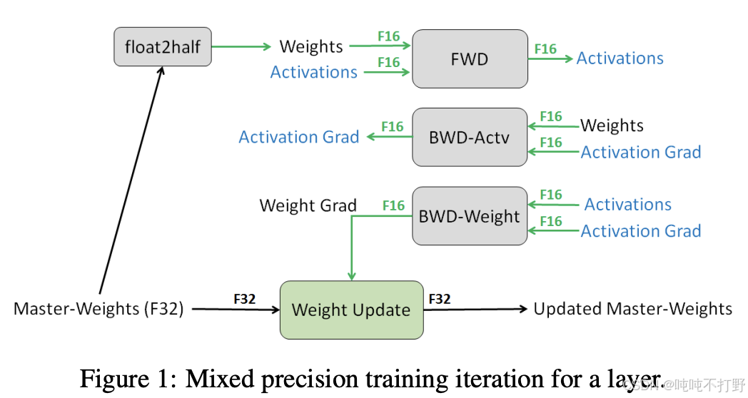
Pytorch has an automatic mixed precision (AMP) library.
- https://pytorch.org/docs/stable/amp.html
- https://docs.nvidia.com/deeplearning/performance/mixed-precision-training/
- 但是需要自己指定哪些部分用什么精度,会有点麻烦
人们正在挑战精度极限。。。有些论文表明,可以在训练的全程都是用FP8
- NVIDIA's Transformer Engine supports FP8 for linear layers
- Use FP8 pervasively throughout training 微软团队. Peng+ 2023------FP8-LM: Training FP8 Large Language Models
另外,之后还会说到,虽然训练对数据精度要求很高,为了保证数值稳定性;但是一旦训练完毕,到了推理阶段,就可以用很大刀阔斧的量化对模型进行瘦身~
X.其他
X. 1. 加减乘除都是用加法器实现的?
好像记得以前学计算机组成原理的时候,提过这么一嘴。
问 Qwen3-Max: 计算机组成原理中,关于加减乘除,本质上都是使用加法实现的,对吗?
答:
不完全对 。虽然现代计算机中的所有算术运算最终都可以通过加法器和逻辑电路的组合来实现 ,但不能简单地说"乘除本质上都是加法"。更准确地说,加法是基础构建模块,其他运算通过加法、移位、控制逻辑等协同实现。
- 加法(Addition)
- 是最基础的算术运算。
- 硬件上由全加器(Full Adder) 构成的加法器电路直接实现。
- 减法通常也通过加法实现(利用补码)。
- 减法(Subtraction)
- 利用二进制补码(Two's Complement) 表示负数。
- 例如:
A - B = A + (-B),而-B就是B的补码。 - 所以减法确实可以转化为加法,共享同一套加法器硬件。
- 乘法(Multiplication)
- 可以 通过重复加法 + 移位(Shift) 实现(如小学手算乘法)。
- 例如:
13 × 5 = 13 + 13 + 13 + 13 + 13(5次加法)。 - 但在二进制中更高效的是:
1101 × 101 = 1101 << 2 + 1101 << 0(利用位移)。
- 例如:
- 但现代CPU不这样做 :
- 使用更高效的算法(如Booth算法、Wallace树、Dadda树等)。
- 专用乘法器硬件单元(Multiplier) ,虽然底层仍由加法器、与门、移位器构成,但不是简单重复加法。
- 所以:乘法可以 用加法实现,但实际硬件不是这样做的,效率太低。
- 可以 通过重复加法 + 移位(Shift) 实现(如小学手算乘法)。
- 除法(Division)
- 可以 通过重复减法 + 移位实现(类似手算除法)。
- 但现代处理器使用更复杂的算法(如SRT除法、Newton-Raphson迭代等)。
- 除法器通常比乘法器更复杂、更慢,很多低端处理器甚至用微码(microcode) 或软件模拟实现除法。
- 所以:除法理论上 可用加/减实现,但实际实现远比"多次加法"复杂。
| 运算 | 是否"本质是加法"? | 实际实现方式 |
|---|---|---|
| 加法 | ✅ 是基础 | 加法器电路 |
| 减法 | ✅(通过补码转加法) | 共用加法器 |
| 乘法 | ❌ 不完全是 | 专用乘法器(含加法+移位+优化算法) |
| 除法 | ❌ 更不是 | 复杂算法或微码,可能调用多次加/减/移位 |
✅ 正确的说法是 :
现代计算机的所有算术运算都建立在加法器、移位器和逻辑门的基础上,加法是最核心的构建模块,但乘除不是"简单地用加法实现",而是通过更高效的专用电路或算法完成。
X.2 动量类的优化算法
1. 带momentum的SGD
直接看pytorch的网页说明:
- torch.optim->SGD
- On the importance of initialization and momentum in deep learning
- 谈谈优化算法之一(动量法、Nesterov法、自然梯度法)
- 11.6. 动量法