使用matlab symbolic toolbox进行拉格朗日建模,并转为LTI模型
Matlab
%% Cart-Pole Lagrangian modeling + symbolic linearization (upright, theta=0)
clear; clc;
syms x dx ddx real
syms th dth ddth real
syms M m l g u real

% --- Generalized coordinates
q   = [x;  th];
dq  = [dx; dth];
ddq = [ddx; ddth];

% --- Kinetic & Potential energy
% Cart velocity: dx
% Pole mass position: px = x + l*sin(th), pz = l*cos(th)
% Velocities:
vpx = dx + l*cos(th)*dth;
vpz = -l*sin(th)*dth;
v2  = vpx^2 + vpz^2;

T_cart = 0.5*M*dx^2;
T_pole = 0.5*m*v2;
T = T_cart + T_pole;

% Potential energy (zero at upright th=0 ⇒ V = m*g*l*(1 - cos(th)))
V = m*g*l*(1 - cos(th));

% Lagrangian
L = T - V;

% --- Generalized forces (only x is actuated by force u)
Q = [u; 0];

% --- Euler-Lagrange: d/dt(dL/ddq) - dL/dq = Q
dLd_dq  = jacobian(L, q).';         % ∂L/∂q
dLd_ddq = jacobian(L, dq).';        % ∂L/∂dq

% Time derivative of dLd_ddq (treat q,dq as functions of time)
% Use total derivative: d/dt = (∂/∂q)*dq + (∂/∂dq)*ddq
d_dt_dLd_ddq = jacobian(dLd_ddq, q)*dq + jacobian(dLd_ddq, dq)*ddq;

EL = d_dt_dLd_ddq - dLd_dq - Q;     % = 0 gives equations of motion

% Solve for accelerations ddq = [ddx; ddth]
sol = solve(EL == 0, ddq);
ddx_expr  = simplify(sol.ddx);
ddth_expr = simplify(sol.ddth);

% --- Build nonlinear state-space: X=[x;dx;th;dth]
f = [
    dx;
    ddx_expr;
    dth;
    ddth_expr
];
g_u = jacobian(f, u);   % input channel (should be a 4x1)
f0  = subs(f, u, 0);    % drift when u=0

% --- Linearize around upright equilibrium: x=0, dx=0, th=0, dth=0, u=0
xeq = [0; 0; 0; 0];
ueq = 0;

A = simplify( subs( jacobian(f, [x, dx, th, dth]), ...
    [x, dx, th, dth, u], [xeq.', ueq] ) );
B = simplify( subs( g_u, [x, dx, th, dth, u], [xeq.', ueq] ) );

% --- Optional: pretty-print A, B
disp('A ='); pretty(A); disp('B ='); pretty(B);

% --- 验证:将A,B化简到常见形式(象征参数不数值化)
A_simplified = simplify(A);
B_simplified = simplify(B);

% --- 如果想代入具体参数,取消注释以下行:
% Mv = 1.0; mv = 0.1; lv = 0.5; gv = 9.81;
% A_num = double(subs(A_simplified, {M,m,l,g}, {Mv,mv,lv,gv}));
% B_num = double(subs(B_simplified, {M,m,l}, {Mv,mv,lv}));
latex代码
% ==========================================================
% Cart-Pole (Simplified) Lagrangian Modeling + Linearization
% ==========================================================
\section{Simplified Cart--Pole Model and Symbolic Linearization}
\label{sec:cartpole_model}
To validate the modeling and control pipeline in a minimal setting, a classical cart--pole
system is considered. The model is derived using the Euler--Lagrange method and then
symbolically linearized around the upright equilibrium.
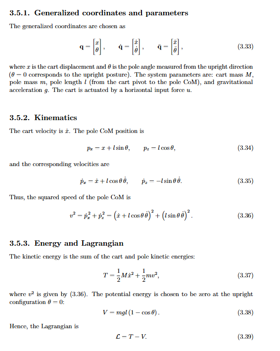
\subsection{Generalized coordinates and parameters}
\label{subsec:cartpole_coordinates}
The generalized coordinates are chosen as
\begin{equation}
\mathbf{q}=
\begin{bmatrix}
x\\ \theta
\end{bmatrix},\qquad
\dot{\mathbf{q}}=
\begin{bmatrix}
\dot{x}\\ \dot{\theta}
\end{bmatrix},\qquad
\ddot{\mathbf{q}}=
\begin{bmatrix}
\ddot{x}\\ \ddot{\theta}
\end{bmatrix},
\end{equation}
where $x$ is the cart displacement and $\theta$ is the pole angle measured from the upright
direction ($\theta=0$ corresponds to the upright posture).
The system parameters are: cart mass $M$, pole mass $m$, pole length $l$ (from the cart pivot to the pole CoM),
and gravitational acceleration $g$. The cart is actuated by a horizontal input force $u$.
\subsection{Kinematics}
\label{subsec:cartpole_kinematics}
The cart velocity is $\dot{x}$. The pole CoM position is
\begin{equation}
p_x = x + l\sin\theta,\qquad
p_z = l\cos\theta,
\end{equation}
and the corresponding velocities are
\begin{equation}
\dot{p}_x=\dot{x}+l\cos\theta\,\dot{\theta},\qquad
\dot{p}_z=-l\sin\theta\,\dot{\theta}.
\end{equation}
Thus, the squared speed of the pole CoM is
\begin{equation}
v^2=\dot{p}_x^{\,2}+\dot{p}_z^{\,2}
=\left(\dot{x}+l\cos\theta\,\dot{\theta}\right)^2+\left(l\sin\theta\,\dot{\theta}\right)^2.
\label{eq:cartpole_v2}
\end{equation}
\subsection{Energy and Lagrangian}
\label{subsec:cartpole_energy}
The kinetic energy is the sum of the cart and pole kinetic energies:
\begin{equation}
T
=\frac{1}{2}M\dot{x}^2+\frac{1}{2}m v^2,
\label{eq:cartpole_T}
\end{equation}
where $v^2$ is given by \eqref{eq:cartpole_v2}.
The potential energy is chosen to be zero at the upright configuration $\theta=0$:
\begin{equation}
V=mgl\left(1-\cos\theta\right).
\label{eq:cartpole_V}
\end{equation}
Hence, the Lagrangian is
\begin{equation}
\mathcal{L}=T-V.
\label{eq:cartpole_L}
\end{equation}
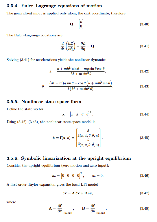
\subsection{Euler--Lagrange equations of motion}
\label{subsec:cartpole_EL}
The generalized input is applied only along the cart coordinate, therefore
\begin{equation}
\mathbf{Q}=
\begin{bmatrix}
u\\ 0
\end{bmatrix}.
\label{eq:cartpole_Q}
\end{equation}
The Euler--Lagrange equations are
\begin{equation}
\frac{d}{dt}\left(\frac{\partial \mathcal{L}}{\partial \dot{\mathbf{q}}}\right)
-\frac{\partial \mathcal{L}}{\partial \mathbf{q}}
=\mathbf{Q}.
\label{eq:cartpole_EL_eq}
\end{equation}
Solving \eqref{eq:cartpole_EL_eq} for accelerations yields the nonlinear dynamics
\begin{equation}
\ddot{x} = \frac{u + ml\dot{\theta}^{2}\sin\theta - mg\sin\theta\cos\theta}{M+m\sin^{2}\theta},
\label{eq:cartpole_ddx}
\end{equation}
\begin{equation}
\ddot{\theta}
=
\frac{(M+m)g\sin\theta - \cos\theta\left(u+ml\dot{\theta}^{2}\sin\theta\right)}
{l\left(M+m\sin^{2}\theta\right)}.
\label{eq:cartpole_ddth}
\end{equation}
\subsection{Nonlinear state-space form}
\label{subsec:cartpole_nonlinear_ss}
Define the state vector
\begin{equation}
\mathbf{x}=
\begin{bmatrix}
x & \dot{x} & \theta & \dot{\theta}
\end{bmatrix}^{\!\top}.
\label{eq:cartpole_state}
\end{equation}
Using \eqref{eq:cartpole_ddx}--\eqref{eq:cartpole_ddth}, the nonlinear state-space model is
\begin{equation}
\dot{\mathbf{x}}=\mathbf{f}(\mathbf{x},u)=
\begin{bmatrix}
\dot{x}\\
\ddot{x}(x,\dot{x},\theta,\dot{\theta},u)\\
\dot{\theta}\\
\ddot{\theta}(x,\dot{x},\theta,\dot{\theta},u)
\end{bmatrix}.
\label{eq:cartpole_ss}
\end{equation}
\subsection{Symbolic linearization at the upright equilibrium}
\label{subsec:cartpole_linearization}
Consider the upright equilibrium (zero motion and zero input):
\begin{equation}
\mathbf{x}_0=
\begin{bmatrix}
0 & 0 & 0 & 0
\end{bmatrix}^{\!\top},\qquad
u_0=0.
\label{eq:cartpole_eq}
\end{equation}
A first-order Taylor expansion gives the local LTI model
\begin{equation}
\delta\dot{\mathbf{x}}=\mathbf{A}\,\delta\mathbf{x}+\mathbf{B}\,\delta u,
\label{eq:cartpole_lti}
\end{equation}
where
\begin{equation}
\mathbf{A}=\left.\frac{\partial \mathbf{f}}{\partial \mathbf{x}}\right|_{(\mathbf{x}_0,u_0)},
\qquad
\mathbf{B}=\left.\frac{\partial \mathbf{f}}{\partial u}\right|_{(\mathbf{x}_0,u_0)}.
\label{eq:cartpole_AB_def}
\end{equation}
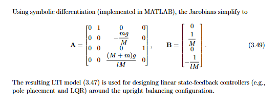
Using symbolic differentiation (implemented in MATLAB), the Jacobians simplify to
\begin{equation}
\mathbf{A}=
\begin{bmatrix}
0 & 1 & 0 & 0\\
0 & 0 & -\dfrac{mg}{M} & 0\\
0 & 0 & 0 & 1\\
0 & 0 & \dfrac{(M+m)g}{lM} & 0
\end{bmatrix},
\qquad
\mathbf{B}=
\begin{bmatrix}
0\\[1mm]
\dfrac{1}{M}\\[1mm]
0\\[1mm]
-\dfrac{1}{lM}
\end{bmatrix}.
\label{eq:cartpole_AB_upright}
\end{equation}
The resulting LTI model \eqref{eq:cartpole_lti} is used for designing linear state-feedback controllers
(e.g., pole placement and LQR) around the upright balancing configuration.