注:本文为 "LSTM" 相关合辑。
英文引文,机翻未校。
中文引文,略作重排。
如有内容异常,请看原文。
What is LSTM - Long Short Term Memory?
什么是 LSTM - 长短期记忆网络?
Last Updated : 23 Dec, 2025
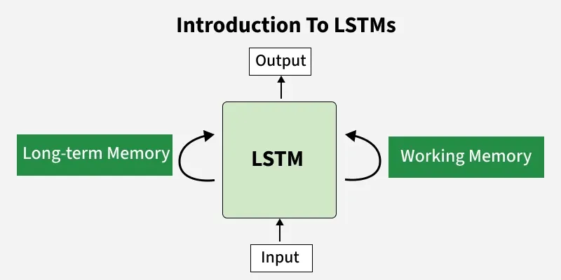
Long Short-Term Memory (LSTM) is an enhanced version of the Recurrent Neural Network (RNN) designed by Hochreiter and Schmidhuber. LSTMs can capture long-term dependencies in sequential data making them ideal for tasks like language translation, speech recognition and time series forecasting. Unlike traditional RNNs which use a single hidden state passed through time LSTMs introduce a memory cell that holds information over extended periods addressing the challenge of learning long-term dependencies.
长短期记忆网络(LSTM)是由霍克赖特(Hochreiter)与施密德胡贝尔(Schmidhuber)提出的循环神经网络(RNN)的改进版本。LSTM 能够捕捉序列数据中的长期依赖关系,因此适用于机器翻译、语音识别、时间序列预测等任务。传统 RNN 仅采用单一隐藏状态随时间传递信息,LSTM 则与之不同,该网络引入记忆单元结构,可长时间存储信息,以此解决学习长期依赖关系时面临的难题。

Problem with Long-Term Dependencies in RNN
循环神经网络(RNN)在处理长期依赖关系时存在的问题
Recurrent Neural Networks (RNNs) are designed to handle sequential data by maintaining a hidden state that captures information from previous time steps. However they often face challenges in learning long-term dependencies where information from distant time steps becomes crucial for making accurate predictions for current state. This problem is known as the vanishing gradient or exploding gradient problem.
循环神经网络(RNN)的设计初衷是通过维持隐藏状态、捕捉历史时间步信息来处理序列数据。但在学习长期依赖关系的过程中,RNN 往往面临阻碍------此类场景下,远期时间步的信息对当前状态的精准预测起到关键作用。这一问题被称为梯度消失或梯度爆炸问题。
-
Vanishing Gradient : When training a model over time, the gradients which help the model learn can shrink as they pass through many steps. This makes it hard for the model to learn long-term patterns since earlier information becomes almost irrelevant.
梯度消失:在模型训练过程中,用于驱动模型学习的梯度值会随着时间步的传递不断衰减。由于早期时间步的信息作用被大幅削弱,模型难以学习到数据中的长期模式。 -
Exploding Gradient : Sometimes gradients can grow too large causing instability. This makes it difficult for the model to learn properly as the updates to the model become erratic and unpredictable.
梯度爆炸:部分情况下,梯度值会异常增大,引发模型训练的不稳定性。模型参数的更新过程因此变得混乱且不可控,进而影响模型的正常学习。
Both of these issues make it challenging for standard RNNs to effectively capture long-term dependencies in sequential data.
上述两类问题的存在,导致标准 RNN 难以有效捕捉序列数据中的长期依赖关系。
LSTM Architecture
LSTM 的网络结构
LSTM architectures involves the memory cell which is controlled by three gates:
LSTM 的网络结构包含记忆单元,该单元的运作由三个门控结构调控:
-
Input gate : Controls what information is added to the memory cell.
输入门:控制哪些信息可以被写入记忆单元。 -
Forget gate : Determines what information is removed from the memory cell.
遗忘门:决定从记忆单元中删除哪些信息。 -
Output gate : Controls what information is output from the memory cell.
输出门:控制从记忆单元中输出哪些信息。
This allows LSTM networks to selectively retain or discard information as it flows through the network which allows them to learn long-term dependencies. The network has a hidden state which is like its short-term memory. This memory is updated using the current input, the previous hidden state and the current state of the memory cell.
这一机制使 LSTM 能够在信息传递过程中选择性地保留或丢弃数据,进而实现对长期依赖关系的学习。网络中存在一种隐藏状态,可视为网络的短时记忆。该状态会结合当前输入、前一时刻的隐藏状态以及记忆单元的当前状态完成更新。
Working of LSTM
LSTM 的工作原理
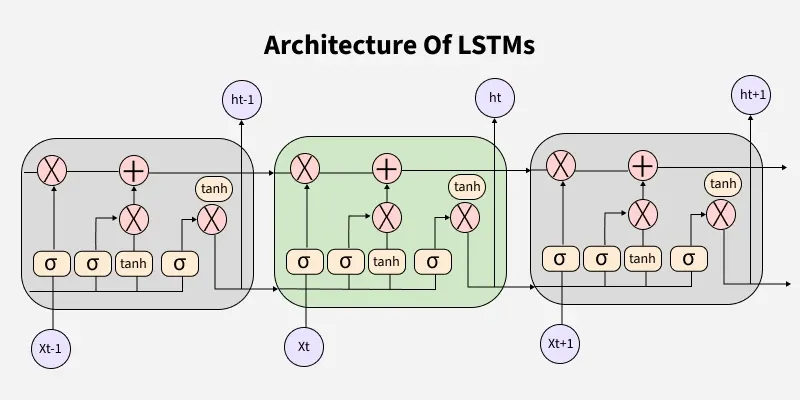
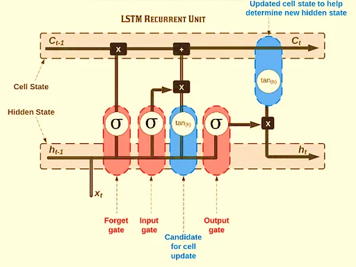
LSTM architecture has a chain structure that contains four neural networks and different memory blocks called cells.
LSTM 采用链式结构,内部包含四个神经网络层与若干被称为记忆单元的存储模块。
LSTM Model
LSTM 模型
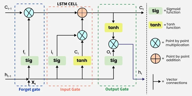
Information is retained by the cells and the memory manipulations are done by the gates. There are three gates -
记忆单元负责存储信息,门控结构负责对存储的信息进行操作。LSTM 包含三个门控结构:
1. Forget Gate
1. 遗忘门
The information that is no longer useful in the cell state is removed with the forget gate. Two inputs x t x_t xt (input at the particular time) and h t − 1 h_{t-1} ht−1 (previous cell output) are fed to the gate and multiplied with weight matrices followed by the addition of bias. The resultant is passed through sigmoid activation function which gives output in range of 0,1. If for a particular cell state the output is 0 or near to 0, the piece of information is forgotten and for output of 1 or near to 1, the information is retained for future use.
遗忘门的作用是清除记忆单元状态中不再具备价值的信息。该门接收两个输入: x t x_t xt(当前时间步的输入数据)与 h t − 1 h_{t-1} ht−1(前一时刻的隐藏状态输出),将输入数据与权重矩阵相乘后叠加偏置项,再将计算结果输入 Sigmoid 激活函数,得到取值范围为 0,1 的输出值。若针对某一单元状态的输出值为 0 或趋近于 0,则对应的信息会被遗忘;若输出值为 1 或趋近于 1,则对应的信息会被保留,用于后续计算。
The equation for the forget gate is:
遗忘门的计算公式如下:
f t = σ ( W f ⋅ h t − 1 , x t + b f ) f_t = \sigma \left( W_f \cdot h_{t-1}, x_t + b_f \right) ft=σ(Wf⋅ht−1,xt+bf)
Where:
其中:
-
W f W_f Wf represents the weight matrix associated with the forget gate.
W f W_f Wf 代表与遗忘门对应的权重矩阵。 -
h t − 1 , x t h_{t-1}, x_t ht−1,xt denotes the concatenation of the current input and the previous hidden state.
h t − 1 , x t h_{t-1}, x_t ht−1,xt 代表对当前输入与前一时刻隐藏状态进行拼接操作。 -
b f b_f bf is the bias with the forget gate.
b f b_f bf 代表遗忘门对应的偏置项。 -
σ \sigma σ is the sigmoid activation function.
σ \sigma σ 代表 Sigmoid 激活函数。
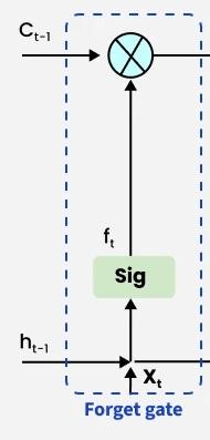
Forget Gate
遗忘门
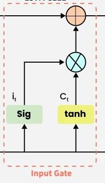
2. Input gate
2. 输入门
The addition of useful information to the cell state is done by the input gate. First the information is regulated using the sigmoid function and filter the values to be remembered similar to the forget gate using inputs h t − 1 h_{t-1} ht−1 and x t x_t xt. Then, a vector is created using tanh function that gives an output from -1 to +1 which contains all the possible values from h t − 1 h_{t-1} ht−1 and x t x_t xt. At last the values of the vector and the regulated values are multiplied to obtain the useful information. The equation for the input gate is:
输入门的作用是向记忆单元状态中写入有用信息。首先,与遗忘门的计算逻辑类似,输入门利用 h t − 1 h_{t-1} ht−1 与 x t x_t xt 两个输入,通过 Sigmoid 函数筛选出需要被记忆的信息;其次,利用 Tanh 函数生成一个取值范围为 -1,1 的向量,该向量涵盖了 h t − 1 h_{t-1} ht−1 与 x t x_t xt 中的全部潜在信息;最后,将该向量与经过筛选的信息相乘,得到待写入记忆单元的有效信息。输入门的计算公式如下:
i t = σ ( W i ⋅ h t − 1 , x t + b i ) i_t = \sigma \left( W_i \cdot h_{t-1}, x_t + b_i \right) it=σ(Wi⋅ht−1,xt+bi)
C ^ t = tanh ( W c ⋅ h t − 1 , x t + b c ) \hat{C}_t = \tanh \left( W_c \cdot h_{t-1}, x_t + b_c \right) C^t=tanh(Wc⋅ht−1,xt+bc)
We multiply the previous state by f t f_t ft effectively filtering out the information we had decided to ignore earlier. Then we add i t ⊙ C ^ t i_t \odot \hat{C}_t it⊙C^t which represents the new candidate values scaled by how much we decided to update each state value.
将记忆单元的前一时刻状态与 f t f_t ft 相乘,可过滤掉之前已确定需要忽略的信息;随后叠加 i t ⊙ C ^ t i_t \odot \hat{C}_t it⊙C^t 这一项,该部分代表经过更新权重缩放后的新候选信息。
C t = f t ⊙ C t − 1 + i t ⊙ C ^ t C_t = f_t \odot C_{t-1} + i_t \odot \hat{C}_t Ct=ft⊙Ct−1+it⊙C^t
where
其中
- ⊙ \odot ⊙ denotes element-wise multiplication
⊙ \odot ⊙ 代表按元素相乘运算 - tanh is activation function
tanh 代表 Tanh 激活函数
Input Gate
输入门
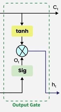
3. Output gate
3. 输出门
The output gate is responsible for deciding what part of the current cell state should be sent as the hidden state (output) for this time step.First, the gate uses a sigmoid function to determine which information from the current cell state will be output. This is done using the previous hidden state h t − 1 h_{t - 1} ht−1 and the current input x t x_t xt:
输出门的作用是决定将当前记忆单元状态中的哪一部分作为本时间步的隐藏状态(输出)。首先,输出门利用前一时刻的隐藏状态 h t − 1 h_{t - 1} ht−1 与当前输入 x t x_t xt,通过 Sigmoid 函数确定当前单元状态中需要输出的信息,计算公式如下:
o t = σ ( W o ⋅ h t − 1 , x t + b o ) o_t = \sigma \left( W_o \cdot h_{t-1}, x_t + b_o \right) ot=σ(Wo⋅ht−1,xt+bo)
Next, the current cell state C t C_t Ct is passed through a tanh activation to scale its values between − 1 -1 −1 and + 1 +1 +1. Finally, this transformed cell state is multiplied element-wise with o t o_t ot to produce the hidden state h t h_t ht:
其次,将当前记忆单元状态 C t C_t Ct 输入 Tanh 激活函数,将其取值缩放至 -1,1 区间;最后,将变换后的单元状态与 o t o_t ot 按元素相乘,得到本时间步的隐藏状态 h t h_t ht,计算公式如下:
h t = o t ⊙ tanh ( C t ) h_t = o_t \odot \tanh(C_t) ht=ot⊙tanh(Ct)
Here:
其中:
-
o t o_t ot is the output gate activation.
o t o_t ot 代表输出门的激活值。 -
C t C_t Ct is the current cell state.
C t C_t Ct 代表当前记忆单元的状态。 -
⊙ \odot ⊙ represents element-wise multiplication.
⊙ \odot ⊙ 代表按元素相乘运算。 -
σ \sigma σ is the sigmoid activation function.
σ \sigma σ 代表 Sigmoid 激活函数。
This hidden state h t h_t ht is then passed to the next time step and can also be used for generating the output of the network.
该隐藏状态 h t h_t ht 会被传递至下一时刻,同时也可用于生成网络的最终输出结果。
Output Gate
输出门
Applications
应用场景
Some of the famous applications of LSTM includes:
LSTM 的典型应用场景如下:
-
Language Modeling : Used in tasks like language modeling, machine translation and text summarization. These networks learn the dependencies between words in a sentence to generate coherent and grammatically correct sentences.
语言建模:应用于语言建模、机器翻译、文本摘要等任务。LSTM 可学习语句中词汇间的依赖关系,从而生成语义连贯、语法正确的文本内容。 -
Speech Recognition : Used in transcribing speech to text and recognizing spoken commands. By learning speech patterns they can match spoken words to corresponding text.
语音识别:应用于语音转文字、语音指令识别等任务。通过学习语音的特征模式,LSTM 能够将语音内容匹配至对应的文本形式。 -
Time Series Forecasting : Used for predicting stock prices, weather and energy consumption. They learn patterns in time series data to predict future events.
时间序列预测:应用于股票价格预测、天气预测、能源消耗预测等任务。LSTM 可学习时间序列数据中的潜在规律,进而实现对未来事件的预测。 -
Anomaly Detection : Used for detecting fraud or network intrusions. These networks can identify patterns in data that deviate drastically and flag them as potential anomalies.
异常检测:应用于欺诈检测、网络入侵检测等任务。LSTM 能够识别数据中存在的显著异常模式,并将其标记为潜在异常事件。 -
Recommender Systems : In recommendation tasks like suggesting movies, music and books. They learn user behavior patterns to provide personalized suggestions.
推荐系统:应用于电影推荐、音乐推荐、书籍推荐等任务。通过学习用户的行为模式,LSTM 可生成符合用户偏好的个性化推荐内容。 -
Video Analysis : Applied in tasks such as object detection, activity recognition and action classification. When combined with Convolutional Neural Networks (CNNs) they help analyze video data and extract useful information.
视频分析:应用于目标检测、行为识别、动作分类等任务。当与卷积神经网络(CNN)结合时,LSTM 可协助完成视频数据的分析工作,并从中提取有效信息。
Suggested Quiz
推荐测试题
5 Questions
5 道题目
What is the main purpose of using LSTM networks over traditional RNNs?
与传统循环神经网络(RNN)相比,使用长短期记忆网络(LSTM)的主要目的是什么?
- A
LSTMs are faster to train
LSTM 的训练速度更快 - B
LSTMs capture long-term dependencies and avoid the vanishing gradient problem
LSTM 能够捕捉长期依赖关系并缓解梯度消失问题 - C
LSTMs are simpler to implement
LSTM 的实现方式更简便 - D
LSTMs are better for image processing tasks
LSTM 更适用于图像处理任务
Which of the following gates is NOT part of the LSTM architecture?
以下哪一种门控结构不属于 LSTM 的网络架构组成部分?
- A
Forget gate
遗忘门 - B
Input gate
输入门 - C
Output gate
输出门 - D
Attention gate
注意力门
What is the role of the "forget gate" in an LSTM network?
长短期记忆网络(LSTM)中,"遗忘门"的作用是什么?
- A
It controls the amount of information to be passed to the output layer
控制传递至输出层的信息量 - B
It decides which information from the previous time step should be discarded
决定丢弃前一时刻的哪些信息 - C
It updates the memory cell with new information
利用新信息更新记忆单元 - D
It produces the final output
生成最终输出结果
What is the key difference between an LSTM and a GRU (Gated Recurrent Unit)?
长短期记忆网络(LSTM)与门控循环单元(GRU)之间的核心区别是什么?
- A
LSTMs are more complex and have more gates than GRUs
LSTM 的结构更复杂,包含的门控数量多于 GRU - B
GRUs require more training data
GRU 需要更多的训练数据 - C
GRUs are slower to train compared to LSTMs
与 LSTM 相比,GRU 的训练速度更慢 - D
LSTMs are not suitable for time series data
LSTM 不适用于时间序列数据
What type of activation function is typically used in the gates of an LSTM?
长短期记忆网络(LSTM)的门控结构中,通常使用哪一种激活函数?
- A
Sigmoid
Sigmoid 函数 - B
Tanh
Tanh 函数 - C
ReLU
ReLU 函数 - D
Softmax
Softmax 函数
题目解析
-
第一题
正确答案:B
解析:传统 RNN 存在梯度消失问题,无法有效捕捉长期依赖关系;LSTM 引入记忆单元与门控结构,可选择性保留或丢弃信息,缓解梯度消失问题,实现对长期依赖的学习。A 错误,LSTM 结构更复杂,训练速度慢于传统 RNN;C 错误,LSTM 实现难度高于传统 RNN;D 错误,LSTM 适用于序列数据,图像处理主流模型为 CNN。
-
第二题
正确答案:D
解析:LSTM 的架构包含遗忘门、输入门、输出门三种门控;注意力门是注意力机制中的结构,不属于 LSTM 固有组件。
-
第三题
正确答案:B
解析:遗忘门的作用是筛选前一时刻记忆单元中的信息,输出值趋近于 0 则丢弃对应信息,趋近于 1 则保留对应信息;A 是输出门的作用,C 是输入门的作用,D 不属于任何门控的直接作用。
-
第四题
正确答案:A
解析:LSTM 包含 3 个门控(遗忘门、输入门、输出门),GRU 仅包含 2 个门控(更新门、重置门),因此 LSTM 结构更复杂;B、C 错误,GRU 结构更简洁,训练速度通常更快,所需训练数据量不一定更多;D 错误,LSTM 是处理时间序列数据的常用模型。
-
第五题
正确答案:A
解析:LSTM 门控结构的输出需要在 0,1 区间内,以此表示信息保留或丢弃的权重,Sigmoid 函数的取值范围恰好为 0,1,因此被用于门控计算;Tanh 函数多用于记忆单元的状态更新,ReLU 与 Softmax 一般不用于 LSTM 门控。
Understanding Long Short-Term Memory (LSTM) Networks
长短期记忆(LSTM)网络概述
Nora Yehia , April 7 2024
LSTMs Long Short-Term Memory is a type of RNNs Recurrent Neural Networkthat can detain long-term dependencies in sequential data.
长短期记忆网络(LSTMs)是一种循环神经网络(RNNs),能够捕捉序列数据中的长期依赖关系。
LSTMs are able to process and analyze sequential data, such as time series, text, and speech.
LSTM 能够处理和分析序列数据,例如时间序列、文本与语音数据。
They use a memory cell and gates to control the flow of information, allowing them to selectively retain or discard information as needed and thus avoid the vanishing gradient problem that plagues traditional RNNs.
该网络通过记忆单元与门控结构控制信息的流动,可根据需求选择性保留或丢弃信息,以此规避传统循环神经网络面临的梯度消失问题。
LSTMs are widely used in various applications such as natural language processing, speech recognition, and time series forecasting.
LSTM 被广泛应用于多种场景,包括自然语言处理、语音识别与时间序列预测等领域。
After reading this post you should know the following:
阅读本文后,你将掌握以下内容:
-
What is Long short-term memory?
什么是长短期记忆网络?
-
Advantages and disadvantages of using LSTM
长短期记忆网络的优缺点
-
How Does Long short-term memory Work?
长短期记忆网络的工作原理
-
Data Loading
数据加载
-
Create Training / Test Data
划分训练集与测试集
-
Perform Preprocessing
执行数据预处理
-
Train a Model
模型训练
-
Measure Model Performance
模型性能评估
What is Long Short-Term Memory?
什么是长短期记忆网络?
Long short-term memory (LSTM) is a type of recurrent neural network (RNN) architecture that is designed to process sequential data and has the ability to remember long-term dependencies.
长短期记忆网络(LSTM)是一种循环神经网络(RNN)架构,专门用于处理序列数据,并且具备捕捉长期依赖关系的能力。
It was introduced by Hochreiter and Schmidhuber in 1997 as a solution to the problem of vanishing gradients in traditional RNNs.
该模型由霍克赖特与施密德胡伯于 1997 年提出,用于解决传统循环神经网络存在的梯度消失问题。
In an LSTM network, each recurrent unit contains a cell state and three types of gates: input, forget, and output gates.
在 LSTM 网络中,每个循环单元包含一个细胞状态与三种门控结构,分别为输入门、遗忘门和输出门。
The input gate controls the flow of new information into the cell state, while the forget gate controls the flow of information that is no longer relevant.
输入门控制新信息流入细胞状态的过程,遗忘门则负责筛选并丢弃不再具有价值的信息。
The output gate controls the flow of information from the cell state to the output of the unit.
输出门用于调控细胞状态向单元输出端传递信息的过程。
The cell state is updated at each time step using a combination of the input, forget, and output gates, as well as the previous cell state.
在每个时间步中,细胞状态会结合输入门、遗忘门、输出门的作用,以及上一时刻的细胞状态完成更新。
This allows the LSTM network to selectively remember or forget information over long periods of time, making it well-suited for tasks such as speech recognition, language translation, and stock price prediction.
这一机制使 LSTM 网络能够在较长时间范围内选择性地记忆或遗忘信息,因此适用于语音识别、机器翻译与股票价格预测等任务。
Overall, LSTMs have become a popular and effective tool in the field of deep learning, and have been used in a wide range of applications across various industries(Figure 0).
总体而言,LSTM 已成为深度学习领域内一种主流且高效的工具,被广泛应用于多个行业的各类场景中(图 0)。
长短期记忆网络结构
Figure 1: Structure of a LSTM 1
图 1:长短期记忆网络结构 1
Advantages and Disadvantages of Using LSTM
长短期记忆网络的优缺点
There are several advantages and disadvantages to using Long Short-Term Memory (LSTM) networks in machine learning and deep learning applications.
在机器学习与深度学习应用中使用长短期记忆(LSTM)网络,存在若干优点与缺点。
Here are some of the key advantages and disadvantages:
以下为具体的优缺点内容:
Advantages:
优点
-
Ability to process sequential data: LSTMs are designed to work with sequential data, such as time series data or natural language text. This makes them well-suited for a wide range of applications, including speech recognition, language translation, and sentiment analysis.
序列数据处理能力:LSTM 专为处理序列数据设计,例如时间序列数据或自然语言文本。这一特性使其适用于多种应用场景,涵盖语音识别、机器翻译与情感分析等领域。
-
Ability to handle long-term dependencies: LSTMs are specifically designed to address the problem of vanishing gradients, which can occur in traditional RNNs when trying to process long sequences. This makes them well-suited for tasks that require processing long-term dependencies, such as predicting stock prices or weather patterns.
长期依赖捕捉能力:LSTM 被专门设计用于解决梯度消失问题,该问题常见于传统循环神经网络处理长序列数据的过程中。因此,LSTM 适用于需要捕捉长期依赖关系的任务,例如股票价格预测与气象模式预测。
-
Memory cell: The memory cell in an LSTM allows the network to selectively remember or forget information over long periods of time, making it more effective at handling complex tasks than other types of RNNs.
记忆单元特性:LSTM 中的记忆单元使网络能够在较长时间范围内选择性地记忆或遗忘信息,相比其他类型的循环神经网络,LSTM 在处理复杂任务时表现更为出色。
Disadvantages:
缺点
-
Training complexity: LSTMs are more complex than traditional RNNs, which can make them more difficult to train. This complexity can also make it harder to interpret and debug an LSTM network.
训练复杂度高:LSTM 的结构比传统循环神经网络更为复杂,这使得模型的训练难度更高,同时也增加了模型解释与调试的难度。
-
Overfitting: LSTMs are prone to overfitting, especially when working with small datasets. This can lead to poor performance on new, unseen data.
过拟合风险:LSTM 容易出现过拟合现象,在处理小规模数据集时尤为明显,这会导致模型在未见过的新数据上表现不佳。
-
Computational cost: LSTMs require more computational resources than traditional RNNs, which can make them slower and more expensive to train.
计算成本高昂:相比传统循环神经网络,LSTM 需要更多的计算资源,这会导致模型训练速度变慢,训练成本增加。
-
Lack of transparency: Like other deep learning models, LSTMs can be difficult to interpret and explain. This can make it harder to understand how the model arrived at its predictions, which can be a concern in some applications.
模型透明度低:与其他深度学习模型类似,LSTM 的决策过程难以解释,使用者很难理解模型生成预测结果的内在逻辑,这在部分应用场景中会成为需要关注的问题。
In summary, LSTMs are a powerful tool for processing sequential data and handling long-term dependencies, but they can be more complex to train and may require more computational resources than other types of RNNs.
综上所述,LSTM 是处理序列数据与捕捉长期依赖关系的有力工具,但相比其他类型的循环神经网络,其训练过程更为复杂,且需要更多的计算资源。
They are best suited for applications where the benefits of their memory cell and ability to handle long-term dependencies outweigh the potential drawbacks.
当记忆单元与长期依赖捕捉能力所带来的收益超过其潜在缺点时,LSTM 能够发挥最佳效果。
How Does Long Short-Term Memory Work?
长短期记忆网络的工作原理
Long Short-Term Memory (LSTM) networks work by processing sequential data through a series of recurrent units, each of which contains a memory cell and three types of gates: input, forget, and output gates.
长短期记忆(LSTM)网络通过一系列循环单元处理序列数据,每个循环单元包含一个记忆单元与三种门控结构,分别为输入门、遗忘门和输出门。
At each time step, the input gate of the LSTM unit determines which information from the current input should be stored in the memory cell.
在每个时间步中,LSTM 单元的输入门决定当前输入数据中的哪些信息需要被存储到记忆单元中。
The forget gate determines which information from the previous memory cell should be discarded, and the output gate controls which information from the current input and the memory cell should be passed to the output of the unit.
遗忘门负责筛选上一时刻记忆单元中需要被丢弃的信息,输出门则控制当前输入与记忆单元中的哪些信息需要传递至单元的输出端。
The memory cell in the LSTM unit is responsible for maintaining long-term information about the input sequence.
LSTM 单元中的记忆单元负责保存输入序列的长期信息。
It does this by selectively updating its contents using the input and forget gates.
记忆单元会借助输入门与遗忘门的作用,选择性地更新自身存储的内容。
The output gate then determines which information from the memory cell should be passed to the next LSTM unit or output layer.
输出门随后决定记忆单元中的哪些信息需要传递至下一个 LSTM 单元或输出层。
During training, the parameters of the LSTM network are learned by minimizing a loss function using backpropagation through time (BPTT).
在训练阶段,LSTM 网络的参数通过时间反向传播(BPTT)算法最小化损失函数来完成学习。
This involves computing the gradients of the loss with respect to the parameters at each time step. Then propagating them backwards through the network to update the parameters.
该过程包括在每个时间步计算损失函数相对于参数的梯度,随后将梯度沿网络反向传播以完成参数更新。
Once the LSTM network has been trained, it can be used for a variety of tasks, such as predicting future values in a time series or classifying text.
LSTM 网络完成训练后,可被用于多种任务,例如时间序列的未来值预测或文本分类任务。
During inference, the input sequence is fed through the network, and the output is generated by the final output layer.
在推理阶段,输入序列被输入至网络中,最终的输出结果由网络的输出层生成。
Overall, LSTMs are a powerful tool for processing sequential data and handling long-term dependencies, making them well-suited for a wide range of applications in machine learning and deep learning(Figure 1).
总体而言,LSTM 是处理序列数据与捕捉长期依赖关系的有力工具,因此适用于机器学习与深度学习领域内的多种应用场景(图 1)。
长短期记忆网络工作原理动态示意图
Figure 2: How a LSTM Work 2
图 2:长短期记忆网络工作原理 2
Implementation Steps of LSTMs
长短期记忆网络的实现步骤
we will discuss how you can use NLP to determine whether the news is real or fake.
本节将介绍如何使用自然语言处理(NLP)技术判断新闻的真伪。
Nowadays, fake news has become a common problem.
如今,虚假新闻已成为一个普遍存在的问题。
Even respected media organizations are known to propagate fake news and are losing credibility.
即便是备受认可的媒体机构,也存在传播虚假新闻的情况,并因此逐渐丧失公信力。
It can be difficult to trust news, because it can be difficult to know whether a news story is real or fake.
公众很难对新闻内容建立信任,原因在于难以辨别一则新闻的真实与否。
First we import the needed libraries
步骤 1:导入所需的库
python
import pandas as pd
import numpy as np
import tensorflow as tf
from tensorflow.keras.layers import Embedding
from tensorflow.keras.preprocessing.sequence import pad_sequences
from tensorflow.keras.models import Sequential
from tensorflow.keras.preprocessing.text import one_hot
from tensorflow.keras.layers import LSTM
from tensorflow.keras.layers import Dense
import nltk
nltk.download('stopwords')
# here we are importing nltk,stopwords and porterstemmer we are using stemming on the text
# we have and stopwords will help in removing the stopwords in the text

#re is regular expressions used for identifying only words in the text and ignoring anything else
import nltk
import re
from nltk.stem.porter import PorterStemmer
from nltk.corpus import stopwords
ps=PorterStemmer()
from sklearn.metrics import classification_report
python
import pandas as pd
import numpy as np
import tensorflow as tf
from tensorflow.keras.layers import Embedding
from tensorflow.keras.preprocessing.sequence import pad_sequences
from tensorflow.keras.models import Sequential
from tensorflow.keras.preprocessing.text import one_hot
from tensorflow.keras.layers import LSTM
from tensorflow.keras.layers import Dense
import nltk
nltk.download('stopwords')
# 代码功能说明:导入自然语言处理工具包 nltk、停用词库 stopwords 与波特词干提取器 PorterStemmer;
# 对文本数据执行词干提取操作,停用词库用于移除文本中的停用词

# 代码功能说明:导入正则表达式库 re,用于筛选文本中的词汇信息,忽略非词汇类内容
import nltk
import re
from nltk.stem.porter import PorterStemmer
from nltk.corpus import stopwords
ps=PorterStemmer()
from sklearn.metrics import classification_report
load the fake news data from FakeData and see the features of the data(Figure2)
从 虚假新闻数据集 中加载数据,并查看数据集的特征信息(图 2)
python
train_df=pd.read_csv(PATH_TO_YOUR_FILE)
# here we are printing first five lines of our train dataset
train_df.head()
python
train_df=pd.read_csv(PATH_TO_YOUR_FILE)
# 代码功能说明:输出训练数据集的前 5 行数据
train_df.head()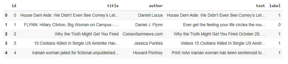
数据集特征展示
Figure 3: Dataset Features
图 3:数据集特征
Data Cleaning and Pre-Processing
步骤 2:数据清洗与预处理
Combining the "title", "author" and "text" columns into a new column called "summary". And also filling any missing values in the data frame with a space
将数据集中的 "title"(标题)、"author"(作者)与 "text"(正文)列合并为一个新列,命名为 "summary"(摘要),并使用空格填充数据框中的缺失值。
python
#filling nan values with space(' ')
train_df.fillna(' ',inplace=True)

#combining title and author,title and summary is formed
train_df['summary']=train_df['title']+' '+train_df['author']+' '+train_df['text']
x=train_df['summary']
y=train_df['label']
python
# 代码功能说明:使用空格填充数据集中的缺失值
train_df.fillna(' ',inplace=True)

# 代码功能说明:合并标题、作者与正文列,生成摘要列
train_df['summary']=train_df['title']+' '+train_df['author']+' '+train_df['text']
x=train_df['summary']
y=train_df['label']
Removing non-alphabetic characters, converting the text to lowercase, tokenizing the text into words, removing stopwords, and stemming the remaining words using the Porter Stemming algorithm. Finally, y joining the preprocessed words back into a string and adding it to the "corpus" list .
执行以下预处理操作:移除文本中的非字母字符、将文本转换为小写形式、对文本进行分词处理、移除分词结果中的停用词、使用波特词干提取算法对剩余词汇执行词干提取,最后将预处理后的词汇重新拼接为字符串,并将其加入语料库(corpus)列表。
python
# here we are creating corpus for the test dataset exactly the same as we created for the
# training dataset
corpus=[]
for i in range(0,len(train_df)):
    review=re.sub('[^a-zA-Z]',' ',x[i])
    review=review.lower()
    review=review.split()
    review=[ps.stem(word) for word in review if not word in stopwords.words('english')]
    review=' '.join(review)
    corpus.append(review)
python
# 代码功能说明:为测试数据集创建语料库,处理流程与训练数据集保持一致
corpus=[]
for i in range(0,len(train_df)):
    review=re.sub('[^a-zA-Z]',' ',x[i])
    review=review.lower()
    review=review.split()
    review=[ps.stem(word) for word in review if not word in stopwords.words('english')]
    review=' '.join(review)
    corpus.append(review)
Preparing text data for using in deep learning model.
为文本数据执行适配深度学习模型的预处理操作:
-
First, setting the vocabulary size to 10000. This means that only the top 10000 most common words in the corpus will be used, and any other words will be discarded.
步骤 1:设置词汇表大小为 10000,即仅保留语料库中出现频率最高的 10000 个词汇,其余词汇将被舍弃。
-
Next, using the
one_hotfunction to convert each word in the corpus into a one-hot encoded vector representation with a length ofvoc_size. This is a common way to represent text data in deep learning models.步骤 2:使用
one_hot函数将语料库中的每个词汇转换为长度为voc_size的独热编码向量,这是深度学习模型中表示文本数据的常用方法。 -
Then, specifying a sentence length of 500, which means that all sentences in the corpus will be padded or truncated to have a length of 500. This is necessary because deep learning models generally expect input data to have a fixed size.
步骤 3:指定句子长度为 500,即对语料库中的所有句子执行填充或截断操作,使其长度统一为 500。深度学习模型通常要求输入数据具有固定尺寸,因此该步骤是必要的。
-
Finally, using the
pad_sequencesfunction to pad the one-hot encoded vectors to the specified length ofsent_length. using the "pre" padding mode, which means that any padding will be added to the beginning of the sequence.步骤 4:使用
pad_sequences函数将独热编码向量填充至指定长度sent_length,采用 "pre" 填充模式,即在序列的开头位置进行填充。 -
Note ,if you want to use a word embedding technique, you can replace the
one_hotfunction with a more sophisticated method such asWord2Vec, GloVe, or FastText.注意事项:若需使用词嵌入技术,可将
one_hot函数替换为更高级的方法,例如 Word2Vec、GloVe 或 FastText。
python
#vocabulary size
voc_size=10000
# TensorFlow has an operation for one-hot encoding
one_hot_reps1=[one_hot(word,voc_size) for word in corpus]
# here we are specifying a sentence length so that every sentence in the corpus will be of same length
sent_length=500
#making all the sentence as equall size vector
#two types of padding pre and post
embedded_docs1=pad_sequences(one_hot_reps1,padding='pre',maxlen=sent_length)
python
# 代码功能说明:定义词汇表大小
voc_size=10000
# 代码功能说明:调用 TensorFlow 内置的独热编码函数
one_hot_reps1=[one_hot(word,voc_size) for word in corpus]
# 代码功能说明:指定句子长度,使语料库中所有句子的长度保持一致
sent_length=500
# 代码功能说明:将所有句子转换为长度相同的向量
# 代码功能说明:填充模式分为两种,分别为前置填充(pre)与后置填充(post)
embedded_docs1=pad_sequences(one_hot_reps1,padding='pre',maxlen=sent_length)
Converting the preprocessed text data and labels into numpy array using the np.array function.
使用 np.array 函数将预处理后的文本数据与标签转换为 NumPy 数组
python
x=np.array(embedded_docs1)

#label should be 0,1 for lstm
y=np.array(y)
python
x=np.array(embedded_docs1)

# 代码功能说明:LSTM 模型要求标签的格式为 0 和 1
y=np.array(y)
Building Models
步骤 3:构建模型
python
#Creating model
from tensorflow.keras.layers import Dropout
import warnings
warnings.filterwarnings('ignore')
embedded_feature_vector=300
nn=Sequential([

    Embedding(voc_size,embedded_feature_vector,input_length=sent_length),
    Dropout(0.5),
    LSTM(199),
    Dropout(0.4),
    Dense(399,activation='relu'),
    Dense(43,activation='relu'),
    Dense(1,activation='sigmoid')])
nn.compile(optimizer='adam',loss='binary_crossentropy',metrics=['accuracy'])
python
# 代码功能说明:构建深度学习模型
from tensorflow.keras.layers import Dropout
import warnings
warnings.filterwarnings('ignore')
embedded_feature_vector=300
nn=Sequential([

    Embedding(voc_size,embedded_feature_vector,input_length=sent_length),
    Dropout(0.5),
    LSTM(199),
    Dropout(0.4),
    Dense(399,activation='relu'),
    Dense(43,activation='relu'),
    Dense(1,activation='sigmoid')])
nn.compile(optimizer='adam',loss='binary_crossentropy',metrics=['accuracy'])
Splitting and Training
步骤 4:数据集划分与模型训练
python
# here we are splitting the data for training and testing the model
from sklearn.model_selection import train_test_split
X_train, X_test, y_train, y_test = train_test_split(x, y, test_size=0.33, random_state=42)

# Train the model on the training data with validation split
nn.fit(X_train, y_train, validation_split=0.2, epochs=50, batch_size=64)
python
# 代码功能说明:划分数据集,用于模型的训练与测试
from sklearn.model_selection import train_test_split
X_train, X_test, y_train, y_test = train_test_split(x, y, test_size=0.33, random_state=42)

# 代码功能说明:使用训练数据训练模型,并设置验证集比例
nn.fit(X_train, y_train, validation_split=0.2, epochs=50, batch_size=64)
Evolution step
步骤 5:模型评估
Predict on test data then show classification report
使用测试数据进行预测,并输出分类报告。
python
y_pred=nn.predict(X_test)
#use threshold or round to the predicted output here use threshold to binary
y_pred=(y_pred>0.5)
y_pred=y_pred.reshape(-1,)
y_pred= np.array(y_pred)
y_test =np.array(y_test)
print(classification_report(y_test, y_pred))
python
y_pred=nn.predict(X_test)
# 代码功能说明:可通过阈值或四舍五入的方式将预测结果转换为二分类形式,此处使用阈值法
y_pred=(y_pred>0.5)
y_pred=y_pred.reshape(-1,)
y_pred= np.array(y_pred)
y_test =np.array(y_test)
print(classification_report(y_test, y_pred))
Then Plot the confusion matrix given the true and predicted labels(Figure3)
基于真实标签与预测标签绘制混淆矩阵(图 3)。
python
from sklearn.metrics import confusion_matrix, classification_report

cm = confusion_matrix(y_test, y_pred)
from matplotlib import pyplot as plt
import seaborn as sn
sn.heatmap(cm, annot=True, fmt='d')
plt.xlabel('Predicted')
plt.ylabel('Truth')
python
from sklearn.metrics import confusion_matrix, classification_report

cm = confusion_matrix(y_test, y_pred)
from matplotlib import pyplot as plt
import seaborn as sn
sn.heatmap(cm, annot=True, fmt='d')
plt.xlabel('Predicted')
plt.ylabel('Truth')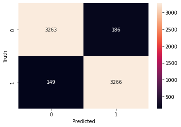
模型混淆矩阵
Figure 4: Model Confusion Matrix
图 4:模型混淆矩阵
Resources:
资源获取
Full source code on Github
完整源代码可访问 Github 仓库
References:
参考文献
Applied LSTM: Use Cases, Types, and Challenges
应用长短期记忆网络:应用场景、类型与挑战
by Sagar Joshi / May 27, 2025
Imagine asking Siri or Google Assistant to set a reminder for tomorrow.
试想你让 Siri 或谷歌助手为明天设置一个提醒事项。
These speech recognition or voice assistant systems must accurately remember your request to set the reminder.
这类语音识别或语音助手系统必须精准记住你设置提醒的指令。
Traditional recurrent networks like backpropagation through time (BPTT) or real-time recurrent learning (RTRL) struggle to remember long sequences because error signals can either grow too big (explode) or shrink too much (vanish) as they move backward through time. This makes learning from a long-term context difficult or unstable.
基于时间的反向传播(BPTT)或实时循环学习(RTRL)等传统循环网络难以记忆长序列,原因是误差信号在时间反向传播过程中会出现幅值过大(梯度爆炸)或幅值过小(梯度消失)的情况。这导致模型难以从长期语境中稳定学习。
Long short-term memory or LSTM networks solve this problem.
长短期记忆网络(LSTM)可解决这一问题。
This artificial neural network type uses internal memory cells to consistently flow important information, allowing machine translation or speech recognition models to remember key details for longer without losing context or becoming unstable.
这类人工神经网络借助内部记忆单元持续传递重要信息,使机器翻译或语音识别模型能够长时间记忆关键细节,且不会丢失语境或出现学习不稳定的情况。
What is long short-term memory (LSTM)?
什么是长短期记忆网络(LSTM)?
Long-short-term memory (LSTM) is an advanced, recurrent neural network (RNN) model that uses a forget, input, and output gate to learn and remember long-term dependencies in sequential data. Its ability to include feedback connections lets it accurately process data sequences instead of individual data points.
长短期记忆网络(LSTM)是一种先进的循环神经网络(RNN)模型,通过遗忘门、输入门和输出门学习并记忆序列数据中的长期依赖关系。该模型具备反馈连接机制,能够对数据序列而非单个数据点进行精准处理。
Invented in 1997 by Sepp Hochreiter and Jürgen Schmidhuber, LSTM addresses RNNs' inability to predict words from long-term memory. As a solution, the gates in an LSTM architecture use memory cells to capture long-term and short-term memory. They regulate the information flow in and out of the memory cell.
LSTM 由塞普·霍克雷特与于尔根·施密德胡伯于 1997 年提出,专门用于解决传统 RNN 无法利用长期记忆预测词汇的问题。LSTM 结构中的各类门控单元借助记忆单元实现长短期记忆的捕获,并调控记忆单元的信息流入与流出过程。
Because of this, users don't experience gradient exploding and vanishing, which usually occurs in standard RNNs. That's why LSTM is ideal for natural language processing (NLP), language translation, speech recognition, and time series forecasting tasks.
这一特性使其避免了标准 RNN 中常见的梯度爆炸与梯度消失问题,因此 LSTM 适用于自然语言处理(NLP)、机器翻译、语音识别以及时间序列预测等任务。
Let's look at the different components of the LSTM architecture.
下文将详细介绍 LSTM 结构的各个组成部分。
LSTM architecture
LSTM 网络结构
The LSTM architecture uses three gates, input, forget, and output, to help the memory cell decide and control what memory to store, remove, and send out. These gates work together to manage the flow of information effectively.
LSTM 结构包含输入门、遗忘门与输出门三类门控单元,协助记忆单元完成信息的存储、清除与输出操作,三类门控协同作用以实现高效的信息流管理。
-
The input gate controls what information to add to the memory cell.
输入门:控制向记忆单元中添加的信息内容
-
The forget gate decides what information to remove from the memory cell.
遗忘门:决定从记忆单元中清除的信息内容
-
The output gate picks the output from the memory cell.
输出门:筛选记忆单元中用于输出的信息内容
This structure makes it easier to capture long-term dependencies.
该结构能够更便捷地捕获数据中的长期依赖关系。
LSTM 网络结构
Source: ResearchGate
来源:研究之门
Input gate
输入门
The input gate decides what information to retain and pass to the memory cell based on the previous output and current sensor measurement data. It's responsible for adding useful information to the cell state.
输入门根据上一时刻的输出与当前时刻的输入数据,决定需要保留并传递至记忆单元的信息,承担向细胞状态中添加有效信息的任务。
Input gate equation:
输入门计算公式:
i t = σ ( W i h t − 1 , x t + b i ) C ^ t = tanh ( W c h t − 1 , x t + b c ) C t = f t ∗ C t − 1 + i t ∗ C ^ t \begin{aligned} i_t &= \sigma \left(W_i h_{t-1}, x_t + b_i\right)\\ \hat{C}t &= \tanh \left(W_c h_{t-1}, x_t + b_c\right)\\ C_t &= f_t * C{t-1} + i_t * \hat{C}_t \end{aligned} itC^tCt=σ(Wiht−1,xt+bi)=tanh(Wcht−1,xt+bc)=ft∗Ct−1+it∗C^t
Where,
其中:
σ \sigma σ is the sigmoid activation function
σ \sigma σ 代表 Sigmoid 激活函数
tanh \tanh tanh represents the tanh activation function
tanh \tanh tanh 代表双曲正切激活函数
W i W_i Wi and W c W_c Wc are weight matrices
W i W_i Wi 与 W c W_c Wc 为权重矩阵
b i b_i bi and b c b_c bc are bias vectors
b i b_i bi 与 b c b_c bc 为偏置向量
h t − 1 h_{t-1} ht−1 is the hidden state in the previous time step
h t − 1 h_{t-1} ht−1 为上一时刻的隐藏状态
x t x_t xt is the input vector at the current time step
x t x_t xt 为当前时刻的输入向量
C ^ t \hat{C}_t C^t is the candidate cell state
C ^ t \hat{C}_t C^t 为候选细胞状态
C t C_t Ct is the cell state
C t C_t Ct 为细胞状态
f t f_t ft is the forget gate vector
f t f_t ft 为遗忘门向量
i t i_t it is the input gate vector
i t i_t it 为输入门向量
∗ * ∗ denotes element-wise multiplication
∗ * ∗ 代表按元素相乘
The input gate uses the sigmoid function to control and filter values to remember. It creates a vector using the tanh function, which produces outputs ranging from -1 to +1 that contain all potential values between h t − 1 h_{t-1} ht−1 and x t x_t xt. Then, the formula multiplies the vector and regulated values to retain valuable information.
输入门通过 Sigmoid 函数控制并筛选需要记忆的信息,同时利用 tanh 函数生成取值范围在 -1 至 +1 之间的向量,该向量涵盖 h t − 1 h_{t-1} ht−1 与 x t x_t xt 之间的所有潜在信息。随后,公式将该向量与经过调控的数值相乘,实现有效信息的保留。
Finally, the equation multiplies the previous cell state element-wise with the forget gate and forgets values close to 0. The input gate then determines which new information from the current input to add to the cell state, using the candidate cell state to identify potential values.
最终,公式将上一时刻的细胞状态与遗忘门向量按元素相乘,清除数值接近 0 的信息。输入门则依据候选细胞状态筛选潜在信息,确定需从当前输入中添加至细胞状态的新信息。
Forget gate
遗忘门
The forget gate controls a memory cell's self-recurrent link to forget previous states and prioritize what needs attention. It uses the sigmoid function to decide what information to remember and forget.
遗忘门通过调控记忆单元的自循环连接,清除历史状态信息并筛选需重点关注的内容,借助 Sigmoid 函数判断信息的保留与清除。
Forget gate equation:
遗忘门计算公式:
F t = σ ( W f h t − 1 , x t + b f ) F_t = \sigma \left(W_f h_{t-1}, x_t + b_f\right) Ft=σ(Wfht−1,xt+bf)
Where,
其中:
σ \sigma σ is the sigmoid activation function
σ \sigma σ 代表 Sigmoid 激活函数
W f W_f Wf is the weight matrix in the forget gate
W f W_f Wf 为遗忘门的权重矩阵
h t − 1 , x t h_{t-1}, x_t ht−1,xt is the sequence of the current input and the previous hidden state
h t − 1 , x t h_{t-1}, x_t ht−1,xt 为当前输入与上一时刻隐藏状态的拼接序列
b f b_f bf is the bias with the forget gate
b f b_f bf 为遗忘门的偏置项
The forget gate formula shows how a forget gate uses a sigmoid function on the previous cell output ( h t − 1 h_{t-1} ht−1) and the input at a particular time ( x t x_t xt). It multiplies the weight matrix with the last hidden state and the current input and adds a bias term. Then, the gate passes the current input and hidden state data through the sigmoid function.
遗忘门计算公式描述了该门控对历史细胞输出( h t − 1 h_{t-1} ht−1)与当前时刻输入( x t x_t xt)执行 Sigmoid 变换的过程:首先将权重矩阵与历史隐藏状态、当前输入的拼接向量相乘,再叠加偏置项,最后将计算结果输入 Sigmoid 函数。
The activation function output ranges between 0 and 1 to decide if part of the old output is necessary, with values closer to 1 indicating importance. The cell later uses the output of f ( t ) f(t) f(t) for point-by-point multiplication.
激活函数的输出值范围为 0 至 1,用于判断历史输出信息的必要性,数值越接近 1 代表对应信息越重要。记忆单元后续会将 f ( t ) f(t) f(t) 的输出结果用于按元素相乘运算。
Output gate
输出门
The output gate extracts useful information from the current cell state to decide which information to use for the LSTM's output.
输出门从当前细胞状态中提取有效信息,确定用于 LSTM 最终输出的内容。
Output gate equation:
输出门计算公式:
o t = σ ( W o h t − 1 , x t + b o ) o_t = \sigma \left(W_o h_{t-1}, x_t + b_o\right) ot=σ(Woht−1,xt+bo)
Where,
其中:
o t o_t ot is the output gate vector at time step t
o t o_t ot 为 t 时刻的输出门向量
W o W_o Wo denotes the weight matrix of the output gate
W o W_o Wo 为输出门的权重矩阵
h t − 1 h_{t-1} ht−1 refers to the hidden state in the previous time step
h t − 1 h_{t-1} ht−1 为上一时刻的隐藏状态
x t x_t xt represents the input vector at the current time step t
x t x_t xt 为 t 时刻的输入向量
b o b_o bo is the bias vector for the output gate
b o b_o bo 为输出门的偏置向量
Output gate equation
o t = σ ( W o h t − 1 , x t + b o ) o_t = \sigma \left(W_o h_{t-1}, x_t + b_o\right) ot=σ(Woht−1,xt+bo)
输出门计算公式
o t = σ ( W o h t − 1 , x t + b o ) o_t = \sigma \left(W_o h_{t-1}, x_t + b_o\right) ot=σ(Woht−1,xt+bo)
Where,
其中:
-
o t o_t ot is the output gate vector at time step t t t
o t o_t ot 为 t t t 时刻的输出门向量 -
W o W_o Wo denotes the weight matrix of the output gate
W o W_o Wo 为输出门的权重矩阵 -
h t − 1 h_{t-1} ht−1 refers to the hidden state in the previous time step
h t − 1 h_{t-1} ht−1 为上一时刻的隐藏状态 -
x t x_t xt represents the input vector at the current time step t t t
x t x_t xt 为 t t t 时刻的输入向量 -
b o b_o bo is the bias vector for the output gate
b o b_o bo 为输出门的偏置向量
It generates a vector by using the tanh function on the cell. Then, the sigmoid function regulates the information and filters the values to be remembered using inputs h t − 1 h_{t-1} ht−1 and x t x_t xt. Finally, the equation multiplies the vector values with regulated values to produce and send an input and output to the next cell.
该门控首先对细胞状态执行 tanh 变换生成向量,再通过 Sigmoid 函数基于输入 h t − 1 h_{t-1} ht−1 与 x t x_t xt 调控并筛选需记忆的信息。最终,公式将生成的向量与调控后的数值相乘,得到输出结果并传递至下一时刻的细胞单元。
Hidden state
隐藏状态
On the other hand, the LSTM's hidden state serves as the network's short-term memory. The network refreshes the hidden state using the input, the current state of the memory cell, and the previous hidden state.
LSTM 的隐藏状态承担网络短期记忆的功能,其更新过程由当前输入、记忆单元的当前状态与上一时刻的隐藏状态共同决定。
Unlike the hidden Markov model (HMM), which predetermines a finite number of states, LSTMs update hidden states based on memory. This hidden state's memory retention ability helps LSTMs overcome long-time lags and tackle noise, distributed representations, and continuous values. That's how LSTM keeps the training model unaltered while providing parameters like learning rates and input and output biases.
隐马尔可夫模型(HMM)预设有限数量的状态,而 LSTM 基于记忆内容更新隐藏状态。隐藏状态的记忆留存能力使 LSTM 能够克服长时间滞后问题,处理噪声数据、分布式表示与连续值数据。这一机制确保 LSTM 在设置学习率、输入输出偏置等参数时,维持训练模型的稳定性。
Hidden layer: the difference between LSTM and RNN architectures
隐藏层:LSTM 与 RNN 结构的差异
The main difference between LSTM and RNN architecture is the hidden layer, a gated unit or cell. While RNNs use a single neural net layer of tanh, LSTM architecture involves three logistic sigmoid gates and one tanh layer. These four layers interact to create a cell's output. The architecture then passes the output and the cell state to the next hidden layer. The gates decide which information to keep or discard in the next cell, with outputs ranging from 0 (reject all) to 1 (include all).
LSTM 与 RNN 结构的主要差异体现在隐藏层,LSTM 的隐藏层为门控单元结构。传统 RNN 的隐藏层仅包含一个 tanh 神经网络层,而 LSTM 隐藏层由三个 Sigmoid 门控与一个 tanh 层构成,四层结构相互作用生成细胞输出。输出结果与细胞状态随后被传递至下一个隐藏层,门控单元依据 0(完全舍弃)至 1(完全保留)的输出值,决定向下一细胞单元传递的信息内容。
Next up: a closer look at the different forms LSTM networks can take.
下文将详细介绍 LSTM 网络的多种变体形式。
Types of LSTM recurrent neural networks
LSTM 循环神经网络的类型
There are X variations of LSTM networks, each with minor changes to the basic architecture to address specific challenges or improve performance. Let's explore what they are.
LSTM 网络存在多种变体,各类变体均通过对基础结构的微调,解决特定场景下的问题或提升模型性能。下文将对其进行逐一介绍。
1. Classic LSTM
1. 经典 LSTM
Also known as vanilla LSTM, the classic LSTM is the foundational model Hochreiter and Schmidhuber promised in 1997.
经典 LSTM 又称标准 LSTM,是霍克雷特与施密德胡伯于 1997 年提出的基础模型。
This model's RNN architecture features memory cells, input gates, output gates, and forget gates to capture and remember sequential data patterns for longer periods. This variation's ability to model long-range dependencies makes it ideal for time series forecasting, text generation, and language modeling.
该模型的循环神经网络结构包含记忆单元、输入门、输出门与遗忘门,能够长期捕获并记忆序列数据的模式特征。其对长距离依赖关系的建模能力,使其适用于时间序列预测、文本生成与语言建模等任务。
2. Bidirectional LSTM (BiLSTM)
2. 双向长短期记忆网络(BiLSTM)
This RNN's name comes from its ability to process sequential data in both directions, forward and backward.
该循环神经网络的命名源于其对序列数据的双向处理能力,可同时实现正向与反向的数据遍历。
Bidirectional LSTMs involve two LSTM networks --- one for processing input sequences in the forward direction and another in the backward direction. The LSTM then combines both outputs to produce the final result. Unlike traditional LSTMs, bidirectional LSTMs can quickly learn longer-range dependencies in sequential data.
双向 LSTM 包含两个独立的 LSTM 网络,分别用于正向与反向处理输入序列,模型最终将两个网络的输出结果融合得到最终预测值。与传统 LSTM 相比,双向 LSTM 能够更高效地学习序列数据中的长距离依赖关系。
BiLSTMs are used for speech recognition and natural language processing tasks like machine translation and sentiment analysis.
双向 LSTM 适用于语音识别及自然语言处理任务,例如机器翻译与情感分析。
3. Gated recurrent unit (GRU)
3. 门控循环单元(GRU)
A GRU is a type of RNN architecture that combines a traditional LSTM's input gate and forget fate into a single update gate. It earmarks cell state positions to match forgetting with new data entry points. Moreover, GRUs also combine cell state and hidden output into a single hidden layer. As a result, they require less computational resources than traditional LSTMs because of the simple architecture.
门控循环单元(GRU)是一种循环神经网络结构,将传统 LSTM 的输入门与遗忘门合并为单一的更新门,通过标记细胞状态位置,实现信息遗忘与新信息输入的匹配。此外,GRU 将细胞状态与隐藏输出整合为单一隐藏层,简洁的结构使其计算资源消耗低于传统 LSTM。
GRUs are popular in real-time processing and low-latency applications that need faster training. Examples include real-time language translation, lightweight time-series analysis, and speech recognition.
GRU 适用于对训练速度要求较高的实时处理与低延迟场景,典型应用包括实时机器翻译、轻量化时间序列分析与语音识别。
4. Convolutional LSTM (ConvLSTM)
4. 卷积长短期记忆网络(ConvLSTM)
Convolutional LSTM is a hybrid neural network architecture that combines LSTM and convolutional neural networks (CNN) to process temporal and spatial data sequences.
卷积 LSTM 是一种混合神经网络结构,融合 LSTM 与卷积神经网络(CNN)的特性,可同时处理时空序列数据。
It uses convolutional operations within LSTM cells instead of fully connected layers. As a result, it's better able to learn spatial hierarchies and abstract representations in dynamic sequences while capturing long-term dependencies.
该模型以卷积运算替代 LSTM 细胞中的全连接层,能够在捕获长期依赖关系的同时,学习动态序列中的空间层级结构与抽象特征表示。
Convolutional LSTM's ability to model complex spatiotemporal dependencies makes it ideal for computer vision applications, video prediction, environmental prediction, object tracking, and action recognition.
卷积 LSTM 对复杂时空依赖关系的建模能力,使其适用于计算机视觉、视频预测、环境预测、目标跟踪与行为识别等应用场景。
5. LSTM with attention mechanism
5. 融合注意力机制的 LSTM
LSTMs using attention mechanisms in their architecture are known as LSTMs with attention mechanisms or attention-based LSTMs.
在结构中引入注意力机制的 LSTM 被称为融合注意力机制的 LSTM,或基于注意力的 LSTM。
Attention in machine learning occurs when a model uses attention weights to focus on specific data elements at a given time step. The model dynamically adjusts these weights based on each element's relevance to the current prediction.
机器学习中的注意力机制,指模型在特定时间步通过注意力权重聚焦于数据的特定元素,并根据各元素与当前预测任务的相关性动态调整权重分配。
This LSTM variant focuses on hidden state outputs to capture fine details and interpret results better. Attention-based LSTMs are ideal for tasks like machine translation, where accurate sequence alignment and strong contextual understanding are crucial. Other popular applications include image captioning and sentiment analysis.
该 LSTM 变体通过关注隐藏状态输出,捕获数据中的细粒度特征并提升结果的可解释性。基于注意力的 LSTM 适用于对序列对齐精度与语境理解能力要求较高的任务,例如机器翻译,同时也可应用于图像描述生成与情感分析等场景。
6. Peephole LSTM
6. 窥视孔 LSTM
A peephole LSTM is another LSTM architecture variant in which input, output, and forget gates use direct connections or peepholes to consider the cell state besides the hidden state while making decisions. This direct access to the cell state enables these LSTMs to make informed decisions about what data to store, forget, and share as output.
窥视孔 LSTM 是另一种 LSTM 结构变体,其输入门、输出门与遗忘门均通过直接连接(窥视孔),在决策过程中同时参考细胞状态与隐藏状态。对细胞状态的直接访问,使该模型能够更合理地决定信息的存储、清除与输出操作。
Peephole LSTMs are suitable for applications that must learn complex patterns and control the information flow within a network. Examples include summary extraction, wind speed precision, smart grid theft detection, and electricity load prediction.
窥视孔 LSTM 适用于需学习复杂模式并调控网络信息流的应用场景,例如文本摘要提取、风速精准预测、智能电网窃电检测与电力负荷预测。
LSTM vs. RNN vs. gated RNN
LSTM、RNN 与门控 RNN 的对比
Recurrent neural networks process sequential data, like speech, text, and time series data, using hidden states to retain past inputs. However, RNNs struggle to remember long sequences from several seconds earlier due to vanishing and exploding gradient problems.
循环神经网络通过隐藏状态留存历史输入信息,实现对语音、文本与时间序列等序列数据的处理。但受梯度消失与梯度爆炸问题影响,RNN 难以记忆几秒前的长序列信息。
LSTMs and gated RNNs address the limitations of traditional RNNs with gating mechanisms that can easily handle long-term dependencies. Gated RNNs use the reset gate and update gate to control the flow of information within the network. And LSTMs use input, forget, and output gates to capture long-term dependencies.
LSTM 与门控 RNN 借助门控机制解决传统 RNN 的缺陷,能够高效处理长期依赖关系。门控 RNN 通过重置门与更新门调控网络信息流,而 LSTM 则利用输入门、遗忘门与输出门捕获长期依赖关系。
| LSTM | RNN | Gated RNN | |
|---|---|---|---|
| Architecture 结构 | Complex with memory cells and multiple gates 结构复杂,包含记忆单元与多个门控 | Simple structure with a single hidden state 结构简单,仅含单一隐藏状态 | Simplified version of LSTM with fewer gates 基于 LSTM 的简化结构,门控数量更少 |
| Gates 门控单元 | Three gates: input, forget, and output 三类门控:输入门、遗忘门、输出门 | No gates 无门控单元 | Two gates: reset and update 两类门控:重置门、更新门 |
| Long-term dependency handling 长期依赖处理能力 | Effective due to memory cell and forget gate 借助记忆单元与遗忘门实现高效处理 | Poor due to vanishing and exploding gradient problem 受梯度消失与爆炸问题影响,处理能力较弱 | Effective, similar to LSTM, but with fewer parameters 处理效果优异,与 LSTM 相近,但参数数量更少 |
| Memory mechanism 记忆机制 | Explicit long-term and short-term memory 具备明确的长短期记忆区分 | Only short-term memory 仅具备短期记忆 | Combines short-term and long-term memory into fewer units 以更少的单元整合长短期记忆 |
| Training time 训练时长 | Slower due to multiple gates and complex architecture 因多门控与复杂结构,训练速度较慢 | Faster to train due to simpler structure 因结构简单,训练速度更快 | Faster than LSTM, slower than RNN due to fewer gates 训练速度快于 LSTM,慢于 RNN,源于更少的门控数量 |
| Use cases 应用场景 | Complex tasks like speech recognition, machine translation, and sequence prediction 适用于复杂任务,如语音识别、机器翻译、序列预测 | Short sequence tasks like stock prediction or simple time series forecasting 适用于短序列任务,如股票预测、简单时间序列预测 | Similar tasks as LSTM but with better efficiency in resource-constrained environments 应用场景与 LSTM 相近,在资源受限环境下具备更高效率 |
LSTM applications
LSTM 的应用场景
LSTM models are ideal for sequential data processing applications like language modeling, speech recognition, machine translation, time series forecasting, and anomaly detection. Let's look at a few of these applications in detail.
LSTM 模型适用于序列数据处理场景,例如语言建模、语音识别、机器翻译、时间序列预测与异常检测。下文将对部分应用场景展开详细介绍。
-
Text generation or language modeling involves learning from existing text and predicting the next word in sequences based on contextual understanding of the previous words. Once you train LSTM models on articles or coding, they can help you with automatic code generation or writing human-like text.
文本生成或语言建模任务,指模型通过学习现有文本数据,基于前文语境预测序列中的下一个词汇。利用文章或代码数据训练 LSTM 模型后,可实现代码自动生成或类人文本写作。
-
Machine translatio n uses AI to translate text from one language to another. It involves mapping a sequence in a language to a sequence in another language. Users can use an encoder-decoder LSTM model to encode the input sequence to a context vector and share translated outputs.
机器翻译技术借助人工智能实现文本的跨语言转换,核心是完成源语言序列到目标语言序列的映射。用户可采用编码 - 解码结构的 LSTM 模型,将输入序列编码为语境向量后,生成对应的翻译输出。 -
Speech recognition system s use LSTM models to process sequential audio frames and understand the dependencies between phonemes. You can also train the model to focus on meaningful parts and avoid gaps between important phonetic components. Ultimately, the LSTM processes inputs using past and future contexts to generate the desired results.
语音识别系统利用 LSTM 模型处理音频帧序列,理解音素之间的依赖关系。通过模型训练,可使其聚焦于音频中的有效信息,忽略重要语音成分之间的无效间隔。最终,LSTM 结合历史与未来语境处理输入数据,生成目标识别结果。 -
Time series forecasting tasks also benefit from LSTMs, which may sometimes outperform exponential smoothing or autoregressive integrated moving average (ARIMA) models. Depending on your training data, you can use LSTMs for a wide range of tasks.
时间序列预测任务同样能借助 LSTM 模型提升性能,部分场景下其预测效果优于指数平滑法或自回归积分滑动平均模型(ARIMA)。根据训练数据的不同,LSTM 可应用于多种预测任务。
For instance, they can forecast stock prices and market trends by analyzing historical data and periodic pattern changes. LSTMs also excel in weather forecasting, using past weather data to predict future conditions more accurately.
例如,通过分析历史数据与周期性模式变化,LSTM 可实现股票价格与市场趋势预测;在气象预测领域,LSTM 利用历史气象数据,能够更精准地预测未来天气状况。
- Anomaly detection applications rely on LSTM autoencoders to identify unusual data patterns and behaviors. In this case, the model trains on normal time series data and can't reconstruct patterns when it encounters anomalous data in the network. The higher the reconstruction error the autoencoder returns, the higher the chances of an anomaly. This is why LSTM models are widely used in fraud detection, cybersecurity, and predictive maintenance.
- 异常检测应用基于 LSTM 自编码器实现异常数据模式与行为的识别。模型首先在正常时间序列数据上完成训练,当输入异常数据时,自编码器无法准确重构数据模式。自编码器的重构误差越大,对应数据存在异常的概率越高。因此,LSTM 模型被广泛应用于欺诈检测、网络安全与预测性维护等领域。
Organizations also use LSTM models for image processing, video analysis, recommendation engines, autonomous driving, and robot control.
各类机构还将 LSTM 模型应用于图像处理、视频分析、推荐系统、自动驾驶与机器人控制等场景。
Drawbacks of LSTM
LSTM 的局限性
Despite having many advantages, LSTMs suffer from different challenges because of their computational complexity, memory-intensive nature, and training time.
尽管具备诸多优势,但受计算复杂度高、内存消耗大与训练周期长等因素影响,LSTM 仍存在若干局限性。
-
Complex architecture: Unlike traditional RNNs, LSTMs are complex as they deal with multiple gates for managing information flow. This complexity means some organizations may find implementing and optimizing LSMNs challenging.
结构复杂度高:与传统 RNN 不同,LSTM 需通过多个门控单元管理信息流,结构相对复杂。这一特性导致部分机构在模型部署与优化过程中面临困难。 -
Overfittin g: LSTMs are prone to overfitting, meaning they may end up generalizing new, unseen data despite being trained well on training data, including noise and outliers. This overfitting happens because the model tries to memorize and match the training data set instead of actually learning from it. Organizations must adopt dropout or regularization techniques to avoid overfitting.
过拟合问题:LSTM 易出现过拟合现象,即模型在包含噪声与异常值的训练数据上表现良好,但对未见过的新数据的泛化能力较弱。过拟合的成因是模型倾向于记忆并拟合训练数据集,而非学习数据中的通用规律。相关机构需采用 Dropout 或正则化技术缓解过拟合问题。 -
Parameter tuning: Tuning LSTM hyperparameters, like learning rate, batch size, number of layers, and units per layer, is time-consuming and requires domain knowledge. You won't be able to improve the model's generalization without finding the optimal configuration for these parameters. That's why using trial and error, grid search, or Bayesian optimization is vital to tune these parameters.
参数调优难度大:LSTM 的超参数调优(如学习率、批次大小、网络层数、每层单元数量等)耗时较长,且需要相关领域知识储备。只有确定超参数的最优配置,才能提升模型的泛化能力。因此,采用试错法、网格搜索或贝叶斯优化等方法进行参数调优至关重要。 -
Lengthy training time: LSTMs involve multiple gates and memory cells. This complexity means you must train the model for many computations, making the training process resource-intensive. Plus, LSTMs need large datasets to learn how to adjust weights for loss minimization iteratively, another reason training takes longer.
训练周期长:LSTM 包含多个门控与记忆单元,结构复杂性导致模型训练过程需执行大量计算,消耗较多计算资源。此外,LSTM 需要基于大规模数据集,通过迭代调整权重以最小化损失函数,这也是训练周期较长的原因之一。 -
Interpretability challenges: Many consider LSTMs as black boxes, meaning it's difficult to interpret how LSTMs make predictions based on various parameters and their complex architecture. Unlike traditional RNNs, you can't trace back the reasoning behind predictions, which may be crucial in industries like finance or healthcare.
可解释性差:LSTM 常被视为"黑箱模型",受复杂结构与多参数影响,其预测决策过程难以被解释。与传统 RNN 不同,LSTM 的预测结果无法追溯明确的推理过程,这一特性使其在金融、医疗等对模型可解释性要求较高的行业中应用受限。
Despite these challenges, LSTMs remain the go-to choice for tech companies, data scientists, and ML engineers looking to handle sequential data and temporal patterns where long-term dependencies matter.
尽管存在上述局限性,在处理需考虑长期依赖关系的序列数据与时序模式时,LSTM 仍是科技企业、数据科学家与机器学习工程师的首选模型。
Next time you ask Siri or Alexa, thank LSTM for the magic
下次使用 Siri 或 Alexa 时,别忘了感谢 LSTM 带来的智能体验
Next time you chat with Siri or Alexa, remember: LSTMs are the real MVPs behind the scenes.
下次与 Siri 或 Alexa 对话时请记住:LSTM 才是幕后的核心技术支撑。
They help you overcome the challenges of traditional RNNs and retain critical information. LSTM models tackle information decay with memory cells and gates, both crucial for maintaining a hidden state that captures and remembers relevant details over time.
LSTM 帮助用户克服传统 RNN 的缺陷,实现关键信息的长效留存。通过记忆单元与门控单元的协同作用,LSTM 解决了信息衰减问题,维持能够长期捕获并记忆相关细节的隐藏状态。
While already foundational in speech recognition and machine translation, LSTMs are increasingly paired with models like XGBoost or Random Forests for smarter forecasting.
LSTM 已成为语音识别与机器翻译领域的基础模型,同时其与极端梯度提升(XGBoost)、随机森林等模型的融合应用,也进一步提升了预测任务的智能化水平。
With transfer learning and hybrid architectures gaining traction, LSTMs continue to evolve as versatile building blocks in modern AI stacks.
随着迁移学习与混合架构的兴起,LSTM 持续发展,成为现代人工智能技术体系中灵活多变的基础组件。
As more teams look for models that balance long-term context with scalable training, LSTMs quietly ride the wave from enterprise ML pipelines to the next generation of conversational AI.
当越来越多的团队寻求兼顾长期语境理解与可扩展训练的模型时,LSTM 正悄然推动技术变革,从企业级机器学习流水线逐步应用于下一代对话式人工智能系统。
Looking to use LSTM to get helpful information from massive unstructured documents? Get started with this guide on named entity recognition (NER) to get the basics right.
使用 LSTM 进行多变量时间序列预测
deephub 原创于 2022-01-11 10:16:44 发布
本文介绍基于 LSTM 实现多变量时间序列预测的方法,涵盖理论与实操,将通过 Python 完成股票价格预测任务,并提供端到端完整代码及详细解析。
文章将先阐述两大基础理论:时间序列分析定义、LSTM 基础原理。
一、时间序列分析
时间序列表示基于时间先后顺序排列的一组数据集合,时间粒度可定义为秒、分钟、小时、日、周、月、年等单位。时间序列的特征为:未来时刻的数值依赖于历史时刻的数值。
在实际应用场景中,时间序列分析主要分为两类:
- 单变量时间序列
- 多变量时间序列
1.1 单变量时间序列
单变量时间序列数据仅包含单一特征列,预测过程仅基于该列的历史数值完成,未来值的推导仅依赖自身的历史规律。

如上图所示,数据结构仅包含单列特征,目标预测值仅由该列的历史数据决定。
1.2 多变量时间序列
多变量时间序列数据包含多个不同维度的特征列,目标预测值会同时依赖多个特征的历史数据与自身的历史规律。

如上图所示,数据结构包含多列特征维度,预测目标列(图中为 c o u n t \mathbf{count} count)的数值,需要综合所有特征列的历史信息完成推导。
在该类数据结构中,目标列 c o u n t \mathbf{count} count 的数值不仅由自身历史值决定,同时受其余特征列的数值影响。因此对目标值进行预测时,必须纳入包含目标列在内的全部特征维度。
1.3 多变量时间序列预测的匹配规则
在多变量时间序列的建模与预测阶段,存在固定的输入维度匹配规则:
若训练阶段的数据集包含 5 5 5 列特征: f e a t u r e 1 , f e a t u r e 2 , f e a t u r e 3 , f e a t u r e 4 , t a r g e t \\mathbf{feature}_1, \\mathbf{feature}_2, \\mathbf{feature}_3, \\mathbf{feature}_4, \\mathbf{target} feature1,feature2,feature3,feature4,target,则在预测阶段,需要为模型输入对应时刻的 4 4 4 列特征值: f e a t u r e 1 , f e a t u r e 2 , f e a t u r e 3 , f e a t u r e 4 \\mathbf{feature}_1, \\mathbf{feature}_2, \\mathbf{feature}_3, \\mathbf{feature}_4 feature1,feature2,feature3,feature4,方可完成目标值的预测。
二、LSTM 基础原理
本文不对 LSTM 的原理展开深度推导,仅给出特性说明,如需学习完整原理,可参考相关专项文献。
LSTM(Long Short-Term Memory)属于循环神经网络(RNN)的改进网络结构,其能力为有效处理数据的长期依赖关系。
循环神经网络的逻辑为:模型可记忆历史输入信息,并将历史信息与当前输入结合完成运算,该特性与人类的时序认知逻辑一致(如通过电影的前序剧情理解后续情节)。但传统 RNN 存在显著缺陷:在处理长序列数据时,易出现梯度消失问题,导致模型无法学习到长期的序列依赖关系。LSTM 网络通过门控机制的设计,从结构层面解决了该问题,具备捕捉长序列依赖的能力。
三、基于 Python 的 LSTM 多变量时间序列预测实现
3.1 导入所需依赖库
python
import numpy as np
import pandas as pd
from matplotlib import pyplot as plt
from tensorflow.keras.models import Sequential
from tensorflow.keras.layers import LSTM
from tensorflow.keras.layers import Dense, Dropout
from sklearn.preprocessing import MinMaxScaler
from keras.wrappers.scikit_learn import KerasRegressor
from sklearn.model_selection import GridSearchCV
3.2 数据集加载与基础探查
加载数据集并查看数据的头部与尾部信息,确认数据的格式与时间跨度:
python
df = pd.read_csv("train.csv", parse_dates=["Date"], index_col=[0])
df.head()
python
df.tail()
数据集说明
本实验采用的数据集为谷歌股票交易数据,时间跨度为 2001 − 01 − 25 ∼ 2021 − 09 − 29 2001-01-25 \sim 2021-09-29 2001−01−25∼2021−09−29,数据的采样频率为日度 。可根据需求将时间频率转换为工作日( ′ B ′ \mathbf{'B'} ′B′)或自然日( ′ D ′ \mathbf{'D'} ′D′),本实验保留原始时间格式即可。
本次实验的预测目标为数据集中 O p e n \mathbf{Open} Open 列的数值,该列为模型的目标特征列。
查看数据集的维度信息:
python
df.shape
(5203, 5)
3.3 时序数据的训练集与测试集划分
时间序列数据的划分禁止随机打乱 ,必须遵循时间先后顺序 的原则,避免破坏数据的时序依赖关系。本实验按 8 : 2 8:2 8:2 的比例划分训练集与测试集:
python
test_split = round(len(df)*0.20)
df_for_training = df[:-1041]
df_for_testing = df[-1041:]
print(df_for_training.shape)
print(df_for_testing.shape)

(4162, 5)
(1041, 5)
3.4 数据标准化处理
股票数据的各特征列数值跨度差异较大,未标准化的数据会导致模型的收敛速度降低、预测精度下降。本实验采用 M i n M a x S c a l e r \mathbf{MinMaxScaler} MinMaxScaler 完成数据的归一化处理,将所有特征的数值映射至区间 0 , 1 0,1 0,1,也可选用 S t a n d a r d S c a l e r \mathbf{StandardScaler} StandardScaler 完成标准化操作。
python
scaler = MinMaxScaler(feature_range=(0,1))
df_for_training_scaled = scaler.fit_transform(df_for_training)
df_for_testing_scaled = scaler.transform(df_for_testing)
df_for_training_scaled
3.5 构造时序监督数据集(X, Y)
该步骤为时序预测的关键环节,需将一维的时序数据转换为模型可训练的监督学习格式,逻辑为:使用历史 n n n 个时间步的全特征数据,预测下一个时间步的目标特征值。
python
def createXY(dataset, n_past):
    dataX = []
    dataY = []
    for i in range(n_past, len(dataset)):
        dataX.append(dataset[i - n_past:i, 0:dataset.shape[1]])
        dataY.append(dataset[i,0])
    return np.array(dataX), np.array(dataY)

trainX, trainY = createXY(df_for_training_scaled, 30)
testX, testY = createXY(df_for_testing_scaled, 30)
函数逻辑说明
参数 n p a s t = 30 n_{\mathbf{past}} = 30 npast=30 表示:使用过去 30 个时间步的全部特征数据,预测第 31 个时间步的目标特征值 ( O p e n \mathbf{Open} Open 列,对应索引为 0 0 0)。
循环逻辑拆解:
- 当 i = 30 i=30 i=30 时, d a t a X \mathbf{dataX} dataX 中存入数据集的 0 : 30 , 0 : 5 0:30, 0:5 0:30,0:5 切片,即前 30 行的全部 5 列特征;
- 当 i = 30 i=30 i=30 时, d a t a Y \mathbf{dataY} dataY 中存入数据集的 30 , 0 30, 0 30,0 数值,即第 31 行的目标特征值;
- 循环完成后, d a t a X \mathbf{dataX} dataX 存储所有的输入特征序列, d a t a Y \mathbf{dataY} dataY 存储对应的预测目标值,最终转换为 n d a r r a y \mathbf{ndarray} ndarray 格式供 LSTM 训练。
查看构造完成的数据集维度:
python
print("trainX Shape-- ",trainX.shape)
print("trainY Shape-- ",trainY.shape)

(4132, 30, 5)
(4132,)

print("testX Shape-- ",testX.shape)
print("testY Shape-- ",testY.shape)

(1011, 30, 5)
(1011,)
维度含义说明:
- t r a i n X : ( 4132 , 30 , 5 ) \mathbf{trainX}: (4132, 30, 5) trainX:(4132,30,5) 表示:共构造 4132 4132 4132 组训练样本,每组样本包含 30 30 30 个时间步,每个时间步包含 5 5 5 个特征维度;
- t r a i n Y : ( 4132 , ) \mathbf{trainY}: (4132,) trainY:(4132,) 表示:每组训练样本对应 1 个目标预测值,共 4132 4132 4132 个标签值。
样本的时序滑动逻辑如下:
t r a i n X 0 : 30 , 0 : 5 → t r a i n Y 30 , 0 t r a i n X 1 : 31 , 0 : 5 → t r a i n Y 31 , 0 t r a i n X 2 : 32 , 0 : 5 → t r a i n Y 32 , 0 \begin{align} \mathbf{trainX}0:30,0:5 &\rightarrow \mathbf{trainY}30,0 \\ \mathbf{trainX}1:31,0:5 &\rightarrow \mathbf{trainY}31,0 \\ \mathbf{trainX}2:32,0:5 &\rightarrow \mathbf{trainY}32,0 \\ \end{align} trainX0:30,0:5trainX1:31,0:5trainX2:32,0:5→trainY30,0→trainY31,0→trainY32,0
查看单组样本的具体内容:
python
print("trainX[0]-- \n",trainX[0])
print("trainY[0]-- ",trainY[0])
3.6 构建 LSTM 模型并完成超参数寻优
本实验通过 G r i d S e a r c h C V \mathbf{GridSearchCV} GridSearchCV 完成模型的超参数调优,选取最优的训练参数组合构建最终模型:
python
def build_model(optimizer):
    grid_model = Sequential()
    grid_model.add(LSTM(50, return_sequences=True, input_shape=(30,5)))
    grid_model.add(LSTM(50))
    grid_model.add(Dropout(0.2))
    grid_model.add(Dense(1))
    grid_model.compile(loss = 'mse', optimizer = optimizer)
    return grid_model

grid_model = KerasRegressor(build_fn=build_model, verbose=1, validation_data=(testX,testY))

parameters = {'batch_size' : [16,20],
              'epochs' : [8,10],
              'optimizer' : ['adam','Adadelta'] }

grid_search  = GridSearchCV(estimator = grid_model,
                            param_grid = parameters,
                            cv = 2)
模型结构说明
- 输入层维度为 ( 30 , 5 ) (30,5) (30,5),与 t r a i n X \mathbf{trainX} trainX 的单样本维度严格匹配,即 ( t i m e s t e p , f e a t u r e d i m ) (\mathbf{time_step}, \mathbf{feature_dim}) (timestep,featuredim);
- 堆叠两层 LSTM 网络,神经元数量均为 50 50 50,第一层开启 r e t u r n s e q u e n c e s = T r u e \mathbf{return_sequences=True} returnsequences=True,为下一层 LSTM 输出完整的序列特征;
- 加入 D r o p o u t ( 0.2 ) \mathbf{Dropout}(0.2) Dropout(0.2) 层抑制过拟合,随机丢弃 20 % 20\% 20% 的神经元连接;
- 输出层为全连接层 D e n s e ( 1 ) \mathbf{Dense}(1) Dense(1),输出单个预测值,匹配回归任务的预测需求。
可根据数据集的规模调整模型复杂度:数据集量较大时,可增加 LSTM 神经元数量与训练轮次;也可通过堆叠更多网络层提升模型的拟合能力。
3.7 模型训练
将构造完成的训练集输入模型,执行超参数寻优与模型训练,该过程会遍历所有参数组合,训练耗时相对较长:
python
grid_search = grid_search.fit(trainX,trainY)训练过程中,模型的损失值会逐步收敛降低:

查看寻优得到的最优超参数组合:
python
grid_search.best_params_

{'batch_size': 20, 'epochs': 10, 'optimizer': 'adam'}
提取最优参数训练完成的模型,作为最终预测模型:
python
my_model = grid_search.best_estimator_.model3.8 基于测试集完成模型预测
使用最优模型对测试集数据进行预测,得到预测值序列:
python
prediction = my_model.predict(testX)
print("prediction\n", prediction)
print("\nPrediction Shape-",prediction.shape)
3.9 预测结果的反标准化还原
模型的输入数据经过 M i n M a x S c a l e r \mathbf{MinMaxScaler} MinMaxScaler 归一化处理,预测结果为标准化后的数值,需执行反标准化操作还原为真实的股票价格。
⚠️ 注意: s c a l e r \mathbf{scaler} scaler 基于 5 列特征完成拟合,反标准化时要求输入数据的列数为 5,直接对预测结果(1 列)执行反标准化会触发维度报错,需通过维度扩充完成适配。
python
# 维度扩充:将1列的预测值复制为5列,匹配scaler的输入维度要求
prediction_copies_array = np.repeat(prediction,5, axis=-1)
pred = scaler.inverse_transform(np.reshape(prediction_copies_array,(len(prediction),5)))[:,0]

# 对测试集真实标签执行同样的反标准化操作
original_copies_array = np.repeat(testY,5, axis=-1)
original = scaler.inverse_transform(np.reshape(original_copies_array,(len(testY),5)))[:,0]
维度扩充的逻辑为:将 1 列的目标特征预测值,在特征维度上复制 4 次,得到 5 列相同数值的矩阵,满足反标准化的输入维度要求;反标准化完成后,仅提取第 0 列(目标特征列)的数值,即为还原后的真实预测值。
查看还原后的预测值与真实值:
python
print("Pred Values-- " ,pred)
print("\nOriginal Values-- " ,original)
3.10 预测结果可视化展示
绘制折线图对比真实值与预测值的拟合效果,直观评估模型的预测精度:
python
plt.plot(original, color = 'red', label = 'Real Stock Price')
plt.plot(pred, color = 'blue', label = 'Predicted Stock Price')
plt.title('Stock Price Prediction')
plt.xlabel('Time')
plt.ylabel('Google Stock Price')
plt.legend()
plt.show()
3.11 未来时间步的股价预测
基于训练完成的模型,对未来 30 30 30 个时间步的股票开盘价进行预测,逻辑为:使用数据集最后 30 30 30 个时间步的全特征数据,滚动预测后续的目标值。
3.11.1 加载预测所需数据
python
# 加载数据集最后30个时间步的历史数据,作为预测的初始输入
df_30_days_past = df.iloc[-30:,:]
df_30_days_past.tail()
python
# 加载未来30个时间步的特征数据(不含目标列Open)
df_30_days_future = pd.read_csv("test.csv", parse_dates=["Date"], index_col=[0])
df_30_days_future
3.11.2 预测数据预处理
为缺失的目标列( O p e n \mathbf{Open} Open)填充默认值 0 0 0,并调整特征列的顺序与训练集一致;对历史数据与未来数据执行标准化处理后,拼接为完整的预测数据集:
python
df_30_days_future["Open"] = 0
df_30_days_future = df_30_days_future[["Open","High","Low","Close","Adj Close"]]
old_scaled_array = scaler.transform(df_30_days_past)
new_scaled_array = scaler.transform(df_30_days_future)

new_scaled_df = pd.DataFrame(new_scaled_array)
new_scaled_df.iloc[:,0] = np.nan
full_df = pd.concat([pd.DataFrame(old_scaled_array),new_scaled_df]).reset_index().drop(["index"],axis=1)
3.11.3 滚动预测未来值
通过循环完成滚动预测,每次预测的结果将作为下一次预测的输入特征,最终得到未来 30 30 30 个时间步的目标值:
python
full_df_scaled_array = full_df.values
all_data = []
time_step = 30
for i in range(time_step,len(full_df_scaled_array)):
    data_x = []
    data_x.append(full_df_scaled_array[i-time_step :i , 0:full_df_scaled_array.shape[1]])
    data_x = np.array(data_x)
    prediction = my_model.predict(data_x)
    all_data.append(prediction)
    full_df.iloc[i,0] = prediction
3.11.4 未来预测值的反标准化还原
python
new_array = np.array(all_data)
new_array = new_array.reshape(-1,1)
prediction_copies_array = np.repeat(new_array,5, axis=-1)
y_pred_future_30_days = scaler.inverse_transform(np.reshape(prediction_copies_array,(len(new_array),5)))[:,0]
print(y_pred_future_30_days)
至此,基于 LSTM 的多变量时间序列预测全流程完成,包含历史数据拟合、测试集验证、未来值预测三个关键环节。

完整可运行代码可参考:https://www.overfit.cn/post/1a36216705f2441b80fca567ea61e365
使用 LSTM 进行简单时间序列预测(入门全流程,包括如何整理输入数据)
eecspan 原创于 2022-03-03 18:22:30 发布
写在前面
在基于 LSTM 开展时间序列预测的实践过程中,多数资料未清晰阐述输入数据的格式规范与预处理逻辑,且部分案例的预测效果存在失真问题。例如:部分案例宣称实现「基于前 30 天数据预测后 10 天数据」,但实际仅完成「逐天滚动预测次日数据」,导致预测效果的视觉表现偏优。
本文参考优质入门文献完成代码实现,并对原文中模糊的逻辑细节进行补充说明。本文不分析 LSTM 模型的拟合效果,仅围绕单变量时间序列,完整阐述输入数据整理、模型定义、模型训练、滚动预测的全流程,确保代码可完整运行并得到合理结果。
一、预测需求定义
给定一组时间序列数据(如连续 100 天的价格数据),数据为单维度特征(每日仅包含价格值),也可扩展为多维度特征(每日包含多个特征值)。本次实验的需求为:基于历史时序数据,预测未来指定长度的时序数值。
二、预测思想
- 首先训练模型的单步预测能力:让模型学习「基于历史数据预测次日数据」的规律;
- 模型训练完成后,执行滚动多步预测 :使用历史数据预测第 114 114 114 天的数值后,将该预测值作为真实值补充至历史数据中,再基于更新后的历史数据预测第 115 115 115 天的数值;
- 重复上述步骤,依次完成后续 30 30 30 天数值的预测,最终得到连续的未来时序预测结果。
三、基于 PyTorch 的 LSTM 模型定义
本实验采用 t o r c h . n n . L S T M ( ) \mathbf{torch.nn.LSTM()} torch.nn.LSTM() 实现网络层,模型的参数定义与结构如下:

input_size -- The number of expected features in the input x
input_size -- 输入x中预期的特征数量hidden_size -- The number of features in the hidden state h
hidden_size -- 隐藏状态h中的特征数量num_layers -- Number of recurrent layers. E.g., setting num_layers=2 would mean stacking two LSTMs together to form a stacked LSTM, with the second LSTM taking in outputs of the first LSTM and computing the final results. Default: 1
num_layers -- 循环层的数量。例如,设置num_layers=2意味着将两个LSTM堆叠起来形成堆叠式LSTM,第二个LSTM接收第一个LSTM的输出并计算最终结果。默认值:1bias -- If False, then the layer does not use bias weights b_ih and b_hh. Default: True
bias -- 若为False,该层不使用偏置权重b_ih和b_hh。默认值:Truebatch_first -- If True, then the input and output tensors are provided as (batch, seq, feature) instead of (seq, batch, feature). Note that this does not apply to hidden or cell states. See the Inputs/Outputs sections below for details. Default: False
batch_first -- 若为True,输入和输出张量的格式为(batch, seq, feature),而非(seq, batch, feature)。注意这不适用于隐藏状态或细胞状态。详情见下方的"输入/输出"部分。默认值:Falsedropout -- If non-zero, introduces a Dropout layer on the outputs of each LSTM layer except the last layer, with dropout probability equal to dropout . Default: 0
dropout -- 若不为0,会在除最后一层外的每个LSTM层的输出上引入Dropout层,丢弃概率等于dropout的值。默认值:0bidirectional -- If True, becomes a bidirectional LSTM. Default: False
bidirectional -- 若为True,将成为双向LSTM。默认值:Falseproj_size -- If > 0, will use LSTM with projections of corresponding size. Default: 0
proj_size -- 若>0,将使用带有对应尺寸投影的LSTM。默认值:0
3.1 LSTM 参数说明
- i n p u t _ s i z e \mathbf{input\_size} input_size:输入数据的特征维度,即单个时间步的特征数量。本实验中单日数据仅包含价格单一特征值,因此 i n p u t _ s i z e = 1 \mathbf{input\_size=1} input_size=1;若单日数据融合开盘价、收盘价、成交量等 n n n 个特征,则对应 i n p u t _ s i z e = n \mathbf{input\_size=n} input_size=n。
- h i d d e n _ s i z e \mathbf{hidden\_size} hidden_size:LSTM 隐藏层状态 h \mathbf{h} h 与细胞状态 c \mathbf{c} c 的特征维度,该参数为手动调优的超参数,数值越大模型特征提取能力越强,需根据数据集复杂度合理设置。
- n u m _ l a y e r s \mathbf{num\_layers} num_layers:堆叠的 LSTM 网络层数,为正整数型超参数。多层堆叠可构建深度循环网络,提升模型拟合能力,但层数过多会增加计算成本,同时极易引发过拟合与梯度消失问题。
3.2 完整模型代码定义
python
import torch
import torch.nn as nn
import numpy as np

class RegLSTM(nn.Module):
    def __init__(self, inp_dim, out_dim, mid_dim, mid_layers):
        super(RegLSTM, self).__init__()
        self.rnn = nn.LSTM(inp_dim, mid_dim, mid_layers)  # LSTM层
        self.reg = nn.Sequential(
            nn.Linear(mid_dim, mid_dim),
            nn.Tanh(),
            nn.Linear(mid_dim, out_dim),
        )  # 回归头,完成特征映射

    def forward(self, x):
        y = self.rnn(x)[0]  # y, (h, c) = self.rnn(x) 仅提取输出序列,舍弃隐状态
        seq_len, batch_size, hid_dim = y.shape
        y = y.view(-1, hid_dim)
        y = self.reg(y)
        y = y.view(seq_len, batch_size, -1)
        return y

    def output_y_hc(self, x, hc):
        y, hc = self.rnn(x, hc)  # 同时返回输出序列与最新的隐状态(h,c)
        seq_len, batch_size, hid_dim = y.size()
        y = y.view(-1, hid_dim)
        y = self.reg(y)
        y = y.view(seq_len, batch_size, -1)
        return y, hc
3.3 模型补充说明
- PyTorch 的 LSTM 输入格式为 s e q _ l e n , b a t c h _ s i z e , i n p u t _ s i z e \boldsymbol{seq\\_len, batch\\_size, input\\_size} seq_len,batch_size,input_size:
示例:input = torch.randn(5, 3, 10)表示:5 个时间步、3 个样本、每个时间步 10 个特征。
- s e q _ l e n seq\_len seq_len:序列长度(时间步);
- b a t c h _ s i z e batch\_size batch_size:批次内的样本数量;
- i n p u t _ s i z e input\_size input_size:单个时间步的特征维度。
-
双前向传播函数的差异:
- f o r w a r d ( ) \mathbf{forward()} forward():仅返回预测结果,舍弃 LSTM 的隐状态 ( h , c ) \boldsymbol{(h,c)} (h,c),每次预测均使用初始隐状态,适用于模型训练阶段;
- KaTeX parse error: Double subscript at position 17: ...mathbf{output_y_̲hc()}:同时返回预测结果与更新后的隐状态 ( h , c ) \boldsymbol{(h,c)} (h,c),下一次预测可将该隐状态传入模型,实现隐状态的连续更新,适用于滚动预测阶段,可提升多步预测的精度。
-
模型参数映射关系:
初始化参数 i n p d i m , m i d d i m , m i d l a y e r s \mathbf{inp_dim, mid_dim, mid_layers} inpdim,middim,midlayers 分别对应 LSTM 的 i n p u t s i z e , h i d d e n s i z e , n u m l a y e r s \mathbf{input_size, hidden_size, num_layers} inputsize,hiddensize,numlayers;输出层维度 o u t d i m \mathbf{out_dim} outdim 为预测值的维度,本实验中为 1(单值预测)。
四、输入数据的整理规范(重点)
4.1 结论
- LSTM 对输入的序列长度(时间步)无强制约束,可根据业务需求选择任意长度的历史数据作为输入;
- 时间序列数据需遵循顺序性原则,禁止打乱;
- 本实验设置 b a t c h s i z e = 1 \mathbf{batch_size}=1 batchsize=1,即单次输入全部训练数据,通过多轮迭代完成训练;
- 实验采用 113 天的历史数据训练模型,最终预测后续 30 天的数值。
4.2 方法一:单序列直接输入训练
4.2.1 数据构造逻辑
将完整的 113 天历史数据作为输入序列 X X X ,将该序列整体后移 1 步得到标签序列 Y Y Y ,即:
X = x 1 , x 2 , x 3 , ... , x 113 Y = x 2 , x 3 , x 4 , ... , x 114 X = x_1, x_2, x_3, \\dots, x_{113} \\ Y = x_2, x_3, x_4, \\dots, x_{114} X=x1,x2,x3,...,x113Y=x2,x3,x4,...,x114
该逻辑的基础为:让模型学习「输入第 t t t 天数据,预测第 t + 1 t+1 t+1 天数据」的规律。若需预测未来第 t + k t+k t+k 天数据,只需将标签序列后移 k k k 步即可。
4.2.2 数据标准化与反标准化函数
时序数据的数值跨度较大,需先完成标准化处理,预测完成后再反标准化还原真实值,同时保留训练集的标准化参数,供测试集与预测阶段使用:
python
def minmaxscaler(x):
    minx = np.amin(x)
    maxx = np.amax(x)
    return (x - minx)/(maxx - minx), (minx, maxx)

def preminmaxscaler(x, minx, maxx):
    return (x - minx)/(maxx - minx)

def unminmaxscaler(x, minx, maxx):
return x * (maxx - minx) + minx- m i n m a x s c a l e r ( ) \mathbf{minmaxscaler()} minmaxscaler():对训练集数据归一化,并返回归一化的最值参数;
- p r e m i n m a x s c a l e r ( ) \mathbf{preminmaxscaler()} preminmaxscaler():使用训练集的最值参数,对测试集/预测数据归一化;
- u n m i n m a x s c a l e r ( ) \mathbf{unminmaxscaler()} unminmaxscaler():反归一化,将预测值还原为真实数值。
4.2.3 数据格式转换(适配 PyTorch LSTM)
PyTorch 的 LSTM 要求输入为三维张量 ,维度定义为: s e q _ l e n , b a t c h _ s i z e , i n p u t _ s i z e \boldsymbol{seq\\_len, batch\\_size, input\\_size} seq_len,batch_size,input_size,具体代码实现如下:
python
bchain = np.array(
    [112., 118., 132., 129., 121., 135., 148., 148., 136., 119., 104.,
     118., 115., 126., 141., 135., 125., 149., 170., 170., 158., 133.,
     114., 140., 145., 150., 178., 163., 172., 178., 199., 199., 184.,
     162., 146., 166., 171., 180., 193., 181., 183., 218., 230., 242.,
     209., 191., 172., 194., 196., 196., 236., 235., 229., 243., 264.,
     272., 237., 211., 180., 201., 204., 188., 235., 227., 234., 264.,
     302., 293., 259., 229., 203., 229., 242., 233., 267., 269., 270.,
     315., 364., 347., 312., 274., 237., 278., 284., 277., 317., 313.,
     318., 374., 413., 405., 355., 306., 271., 306., 315., 301., 356.,
     348., 355., 422., 465., 467., 404., 347., 305., 336., 340., 318.,
     362., 348., 363., 435., 491., 505., 404., 359., 310., 337., 360.,
     342., 406., 396., 420., 472., 548., 559., 463., 407., 362., 405.,
     417., 391., 419., 461., 472., 535., 622., 606., 508., 461., 390.,
     432.], dtype=np.float32)
bchain = bchain[:, np.newaxis]

inp_dim = 1
out_dim = 1
mid_dim = 8
mid_layers = 1
data_x = bchain[:-1, :]
data_y = bchain[+1:, :]

train_size = 113
train_x = data_x[:train_size, :]
train_y = data_y[:train_size, :]

# 数据标准化
train_x, train_x_minmax = minmaxscaler(train_x)
train_y, train_y_minmax = minmaxscaler(train_y)

device = torch.device("cuda" if torch.cuda.is_available() else "cpu")

# 转换为PyTorch的三维张量格式 [seq_len, batch_size, input_size]
batch_x = train_x[:, np.newaxis, :]
batch_y = train_y[:, np.newaxis, :]
batch_x = torch.tensor(batch_x, dtype=torch.float32, device=device)
batch_y = torch.tensor(batch_y, dtype=torch.float32, device=device)
4.3 方法二:滑动窗口构造多序列训练集
该方法通过滑动窗口从原始长序列中截取多个等长的短序列,构造多组训练样本,让模型学习更泛化的时序规律,代码如下:
python
# 滑动窗口构造多序列训练集
train_x_tensor = torch.tensor(train_x, dtype=torch.float32, device=device)
train_y_tensor = torch.tensor(train_y, dtype=torch.float32, device=device)

batch_x = list()
batch_y = list()
window_len = 40
# 步长为3,截取长度为40的序列
for end in range(len(train_x_tensor), window_len, -3):
    batch_x.append(train_x_tensor[end-40:end])
    batch_y.append(train_y_tensor[end-40:end])

# 对齐序列长度并转换为标准格式 [seq_len, batch_size, input_size]
from torch.nn.utils.rnn import pad_sequence
batch_x = pad_sequence(batch_x)
batch_y = pad_sequence(batch_y)
滑动窗口数据格式说明
滑动窗口的逻辑为:将原始长序列切分为多个重叠的短序列,例如原始序列为 1 , 2 , 3 , . . . , 113 1,2,3,...,113 1,2,3,...,113,窗口长度为 40 40 40、步长为 3 3 3,则切分后的序列为 1 − 40 , 4 − 43 , 7 − 46 , . . . 1-40, 4-43, 7-46, ... 1−40,4−43,7−46,...。
切分后的数据集维度为 40 , 25 , 1 \boldsymbol{40, 25, 1} 40,25,1,表示:25 个训练样本、每个样本包含 40 个时间步、每个时间步 1 个特征维度。该格式可让模型并行处理多个序列,提升训练效率与泛化能力。
五、模型训练与预测
5.1 模型训练
python
# 加载模型并定义训练参数
model = RegLSTM(inp_dim, out_dim, mid_dim, mid_layers).to(device)
loss = nn.MSELoss()
optimizer = torch.optim.Adam(model.parameters(), lr=1e-2)

# 模型训练迭代
print("Training......")
for e in range(801):
    out = model(batch_x)
    Loss = loss(out, batch_y)
    optimizer.zero_grad()
    Loss.backward()
    optimizer.step()
    if e % 10 == 0:
        print('Epoch: {:4}, Loss: {:.5f}'.format(e, Loss.item()))
        torch.save(model.state_dict(), './net.pth')
print("Save in:", './net.pth')
训练采用均方误差(MSE)作为损失函数,优化器为 Adam,学习率设置为 1 e − 2 1e-2 1e−2,训练轮次为 800 800 800 轮,每 10 10 10 轮保存一次模型权重。
5.2 滚动多步预测
预测阶段的逻辑为:使用历史数据滚动预测未来值,每次预测的结果补充至历史数据中,作为下一次预测的输入,代码如下:
python
new_data_x = data_x.copy()
new_data_x[train_size:] = 0  # 待预测区域初始化为0
test_len = 40

# 初始化LSTM的隐状态(h,c)
zero_ten = torch.zeros((mid_layers, 1, mid_dim), dtype=torch.float32, device=device)

# 滚动预测后续所有时间步
for i in range(train_size, len(new_data_x)):
    test_x = new_data_x[i-test_len:i, np.newaxis, :]
    test_x = preminmaxscaler(test_x, train_x_minmax[0], train_x_minmax[1])
    batch_test_x = torch.tensor(test_x, dtype=torch.float32, device=device)

    # 首次预测初始化隐状态,后续预测使用更新后的隐状态
    if i == train_size:
        test_y, hc = model.output_y_hc(batch_test_x, (zero_ten, zero_ten))
    else:
        test_y, hc = model.output_y_hc(batch_test_x[-2:], hc)

    # 提取预测值并反标准化还原
    predict_y = test_y[-1].item()
    predict_y = unminmaxscaler(predict_y, train_x_minmax[0], train_y_minmax[1])
    new_data_x[i] = predict_y
5.3 预测结果可视化
绘制折线图对比真实值与预测值,直观展示预测效果:
python
import matplotlib.pyplot as plt
plt.plot(new_data_x, 'r', label='pred')
plt.plot(data_x, 'b', label='real', alpha=0.3)
plt.legend(loc='best')
plt.show()
异常监测------LSTM 时间序列预测 & LSTM 简易原理
nolabel 修改于 2023-05-23 15:28:08
本文详细阐述基于 LSTM 完成时间序列预测的全流程,涵盖数据预处理、模型设计、训练优化与异常判定策略;深度解析 LSTM 的原理,探讨预测滞后性问题的成因与解决方案,并提供损失函数与优化器的选型指南。
一、利用 LSTM 进行时间序列预测的业务背景与完整流程
基于统计学方法( 3 σ 3\sigma 3σ 原则、四分位距法)完成的异常监测,仅适用于数据分布规律稳定的场景。在实际业务中,时序数据的分布规律会随业务迭代发生动态变化,示例如下:
| 时间点 | 原数值 count | 新数值 count |
|---|---|---|
| 2020-01-01 13:00:00 | 267 | 1000 |
| 2020-01-01 13:10:00 | 300 | 0 |
| 2020-01-01 13:20:00 | 261 | 0 |
| 2020-01-01 13:30:00 | 289 | 1023 |
| 2020-01-01 13:40:00 | 235 | 0 |
| 2020-01-01 13:50:00 | 273 | 0 |
| 2020-01-01 14:00:00 | 309 | 1014 |
此时传统统计学方法将失效,若通过人工修改异常判定逻辑,将面临持续迭代的维护成本。因此选用LSTM 深度学习模型 对时序数据的分布规律进行预测,并加入模型自动更新逻辑,实现无需人工干预的自适应异常监测。
1.1 完整业务流程规范
1、原始数据存储
采用 MongoDB 完成时序数据的存储,适配时序数据的高频写入与查询需求。
2、数据预处理
执行标准化的数据清洗操作:剔除节假日无效数据、异常值插值替换、缺失值填充,确保输入模型的数据质量。
3、模型设计及训练
- 训练集:选取近 10 天的时序数据(剔除近 3 天);
- 测试集:选取近 3 天的时序数据;
- 执行多轮超参数优化,确定最优的模型参数与序列长度(历史时间步);
- 训练完成后保存模型权重文件,供线上预测使用。
4、异常判断策略
采用双重异常判定规则,提升异常识别的准确性:
① 参考行业实践,取预测值的 90 % 90\% 90% 分位数作为异常边界,当连续多次触发异常阈值时,推送告警(邮件/微信);
② 基于 3 σ 3\sigma 3σ 原则,当实际值超出预测值的 μ ± 3 σ \mu \pm 3\sigma μ±3σ 区间时,判定为异常。
5、模型自动更新机制
设置双层监控规则,触发任一规则即自动重新训练模型:
- 数据监控:按日粒度计算数据的均值、标准差、中位数、四分位距(IQR),当统计指标的漂移量超过阈值时,判定为数据分布发生变化;
- 模型监控:按日统计模型输出的异常点占比,当异常占比的分布规律发生显著变化时,判定为模型拟合能力下降。
1.2 重要预处理准则
训练集与测试集的标准化需独立执行:训练集的标准化参数(均值、标准差/最值)仅由训练集计算得到,测试集的标准化需复用训练集的参数,禁止将训练集与测试集合并后再标准化,避免数据泄露导致的模型泛化能力下降。
二、LSTM 预测的滞后性问题及解决方案
2.1 滞后性的成因
LSTM 模型在时间序列预测中出现的预测值滞后于真实值,是行业内的常见问题,成因主要分为两类:
- 过拟合导致的滞后:模型过度拟合训练集的历史规律,对新数据的变化不敏感,预测值始终跟随真实值的变化而变化,表现为滞后。该结论来源于 StackOverflow 社区的经典总结;
- 权重偏置导致的滞后:LSTM 模型在训练过程中,对序列的最后一个时间步的权重赋值过高,导致预测值近似等于序列最后一个时间步的数值,表现为对真实值的滞后复现。该结论来源于工程实践总结。
2.2 滞后性的解决方案
针对上述成因,可采取以下优化措施:
- 抑制过拟合:在模型中加入 Dropout 层、L1/L2 正则化,或通过早停(EarlyStopping)终止训练;
- 调整模型结构:减少 LSTM 神经元数量与网络层数,降低模型的拟合能力;
- 优化训练策略:增大批次大小、降低学习率,让模型的收敛过程更平稳;
- 数据增强:对时序数据进行加噪、重采样等增强操作,提升模型的泛化能力。
三、LSTM 原理深度解析
3.1 LSTM 的设计目标
传统循环神经网络(RNN)在处理长序列数据时,会因梯度消失/梯度爆炸 问题,无法学习到序列的长期依赖关系。LSTM 通过门控机制的结构设计,从根本上解决了该问题,具备捕捉长时序依赖的能力。
梯度消失的数学本质:当序列长度 T T T 过大时,损失函数 L L L 对隐藏状态 h t h_t ht 的梯度会随序列长度的增加呈指数级衰减,导致模型无法更新长序列的权重参数。
3.2 LSTM 的四大路径(直观理解)
LSTM 的神经元内部包含四条并行的信息处理路径,分别实现预测、遗忘、筛选、忽视的功能,四条路径协同工作,完成时序信息的记忆与更新。
激活函数的符号定义
- tanh \tanh tanh 双曲正切函数:输出值映射至区间 − 1 , 1 -1,1 −1,1,用于生成候选的记忆信息;
- s i g m o i d \mathbf{sigmoid} sigmoid 逻辑斯蒂函数:输出值映射至区间 0 , 1 0,1 0,1,输出值可理解为「门控的开合程度」, 0 0 0 表示完全关闭, 1 1 1 表示完全开启。
路径一:预测路径(Prediction)
传统 RNN 的逻辑:基于上一时刻的隐藏状态(历史预测)与当前时刻的输入(新信息),计算当前时刻的预测值,该预测值将作为下一时刻的输入特征。该路径是所有循环神经网络的基础。
路径二:遗忘路径(Forgetting)→ 遗忘门
为解决 RNN 的短期记忆问题,LSTM 加入遗忘门,功能为选择性遗忘历史信息:
- 遗忘门通过 s i g m o i d \mathbf{sigmoid} sigmoid 函数生成门控值,输入为上一时刻的隐藏状态与当前时刻的输入;
- 门控值与上一时刻的记忆细胞(Cell State)执行逐元素乘法,门控值越接近 0 0 0,表示越需要遗忘该部分信息;越接近 1 1 1,表示越需要保留该部分信息。
路径三:筛选路径(Selection)→ 输出门
输出门的功能为选择性输出记忆信息:
- 输出门通过 s i g m o i d \mathbf{sigmoid} sigmoid 函数生成门控值,输入为上一时刻的隐藏状态与当前时刻的输入;
- 门控值与当前时刻的记忆细胞执行逐元素乘法,筛选出需要输出的信息,生成当前时刻的隐藏状态;
- 输出门的门控值决定了记忆细胞中的信息有多少可以传递到模型的输出层,门控值为 0 0 0 时,记忆信息仅保存在细胞内部;门控值为 1 1 1 时,记忆信息完全输出。
路径四:忽视路径(Ignoring)→ 输入门
输入门的功能为选择性录入新信息:
- 输入门通过 s i g m o i d \mathbf{sigmoid} sigmoid 函数生成门控值,输入为上一时刻的隐藏状态与当前时刻的输入;
- 门控值与候选记忆细胞(由 tanh \tanh tanh 函数生成)执行逐元素乘法,筛选出需要录入的新信息;
- 筛选后的新信息将与遗忘后的历史信息相加,生成当前时刻的记忆细胞,完成记忆的更新。
3.3 LSTM 的数学公式(工程必知)
LSTM 的所有逻辑均可通过数学公式精准表达,以下为工程实践中最常用的公式,所有符号的定义均遵循行业标准:
1、遗忘门 F t \boldsymbol{F_t} Ft
F t = σ ( W x f X t + W h f H t − 1 + b f ) F_t = \sigma(W_{xf}X_t + W_{hf}H_{t-1} + b_f) Ft=σ(WxfXt+WhfHt−1+bf)
作用:控制上一时刻的记忆细胞 C t − 1 C_{t-1} Ct−1 中有多少信息被保留至当前时刻。
2、输入门 I t \boldsymbol{I_t} It
I t = σ ( W x i X t + W h i H t − 1 + b i ) I_t = \sigma(W_{xi}X_t + W_{hi}H_{t-1} + b_i) It=σ(WxiXt+WhiHt−1+bi)
作用:控制当前时刻的输入 X t X_t Xt 有多少信息被录入至当前时刻的记忆细胞。
3、候选记忆细胞 C ~ t \boldsymbol{\tilde{C}_t} C~t
C ~ t = tanh ( W x c X t + W h c H t − 1 + b c ) \tilde{C}t = \tanh(W{xc}X_t + W_{hc}H_{t-1} + b_c) C~t=tanh(WxcXt+WhcHt−1+bc)
作用:生成当前时刻的候选记忆信息,是对输入数据的特征映射。
4、记忆细胞更新 C t \boldsymbol{C_t} Ct
C t = F t ⊙ C t − 1 + I t ⊙ C ~ t C_t = F_t \odot C_{t-1} + I_t \odot \tilde{C}_t Ct=Ft⊙Ct−1+It⊙C~t
作用:完成记忆细胞的更新, ⊙ \odot ⊙ 表示逐元素乘法,该公式是 LSTM 解决梯度消失的关键。
5、输出门 O t \boldsymbol{O_t} Ot
O t = σ ( W x o X t + W h o H t − 1 + b o ) O_t = \sigma(W_{xo}X_t + W_{ho}H_{t-1} + b_o) Ot=σ(WxoXt+WhoHt−1+bo)
作用:控制当前时刻的记忆细胞 C t C_t Ct 中有多少信息被传递到隐藏状态 H t H_t Ht。
6、隐藏状态输出 H t \boldsymbol{H_t} Ht
H t = O t ⊙ tanh ( C t ) H_t = O_t \odot \tanh(C_t) Ht=Ot⊙tanh(Ct)
作用:生成当前时刻的隐藏状态,作为模型的输出特征,供后续的全连接层使用。
3.4 门控机制的总结
- LSTM 的三个门控(遗忘门 F t F_t Ft、输入门 I t I_t It、输出门 O t O_t Ot)均由 s i g m o i d \mathbf{sigmoid} sigmoid 函数生成,输出值的区间为 0 , 1 0,1 0,1,完美适配「门控开合程度」的物理意义;
- 遗忘门控制「历史信息的保留比例」,输入门控制「新信息的录入比例」,输出门控制「记忆信息的输出比例」;
- 所有门控的权重参数 W W W 与偏置参数 b b b 均由模型在训练过程中自动学习得到,模型可自适应调整门控策略,从而拟合不同的时序规律;
- 记忆细胞 C t C_t Ct 是 LSTM 的关键,其更新过程无梯度衰减,是模型能捕捉长时序依赖的根本原因。
3.5 原理具象化示例
以简单的文本序列预测为例,直观理解 LSTM 的门控机制:
给定童书的三类句子:「道格看见珍。」、「珍看见小点。」、「小点看见道格。」,对句子进行 One-Hot 编码后输入 LSTM 模型。
当输入序列为「珍看见小点。道格」时,模型的处理逻辑如下:
- 输入「道格」后,模型的初步预测为「看见」与「非道格」;
- 遗忘门筛选出历史信息中的「名字」相关特征,遗忘「看见」相关特征;
- 输入门录入新信息「道格」,生成候选记忆「道格→看见」;
- 输出门筛选出「看见」作为最终预测值;
- 后续输入「看见」时,模型的遗忘门遗忘历史的「看见」特征,保留「道格」特征,最终预测出「珍」或「小点」。
该示例清晰展示了 LSTM 的门控机制如何通过选择性的记忆与遗忘,完成对序列规律的学习。
四、LSTM 模型的参数详解
4.1 模型参数定义
以下为 Keras 框架中 LSTM 模型的经典实现代码,所有参数均为工程实践中的常用配置:
python
from tensorflow.keras.models import Sequential
from tensorflow.keras.layers import LSTM, Dropout, Dense

model = Sequential()
model.add(LSTM(neurons, input_shape=(None,1)))
model.add(Dropout(dropout_value))
model.add(Dense(1))
model.compile(loss='mean_squared_error', optimizer='adam')
model.fit(train_x, train_y, epochs=epochs, batch_size=batch_size, verbose=verbose)
4.2 关键参数详解
1、LSTM 层参数
- n e u r o n s \boldsymbol{neurons} neurons:LSTM 层的神经元数量,决定模型的拟合能力,神经元越多,拟合能力越强,但越易过拟合。工程实践中建议从 32 、 50 、 64 32、50、64 32、50、64 开始尝试。
- i n p u t _ s h a p e = ( t i m e s t e p s , i n p u t _ d i m ) \boldsymbol{input\_shape=(timesteps, input\_dim)} input_shape=(timesteps,input_dim):输入数据的维度, t i m e s t e p s \mathbf{timesteps} timesteps 为序列长度(时间步), i n p u t d i m \mathbf{input_dim} inputdim 为单个时间步的特征维度。若设置为 ( N o n e , i n p u t d i m ) \mathbf{(None, input_dim)} (None,inputdim),表示支持任意长度的序列输入。
2、Dropout 层参数
- d r o p o u t _ v a l u e \boldsymbol{dropout\_value} dropout_value:随机丢弃的神经元比例,取值范围为 0 , 1 0,1 0,1,默认值为 0 0 0。作用为抑制过拟合,工程实践中建议取值为 0.1 ∼ 0.3 0.1 \sim 0.3 0.1∼0.3。
3、编译阶段参数
- l o s s \boldsymbol{loss} loss:损失函数,决定模型的优化方向,不同的任务类型需选择对应的损失函数;
- o p t i m i z e r \boldsymbol{optimizer} optimizer:优化器,决定模型的参数更新策略,常用的优化器有 Adam、SGD、Adadelta 等。
4、训练阶段参数
- e p o c h s \boldsymbol{epochs} epochs:训练轮次,即整个训练集被模型学习的次数。轮次过多易过拟合,轮次过少易欠拟合;
- b a t c h _ s i z e \boldsymbol{batch\_size} batch_size:批次大小,即单次训练中模型处理的样本数量。批次越大,训练越稳定,但内存占用越高;
- v e r b o s e \boldsymbol{verbose} verbose:日志输出模式,取值为 0 、 1 、 2 0、1、2 0、1、2,分别表示无日志、进度条日志、单行日志。
4.2 训练参数的关系定义
为避免参数混淆,给出明确的数学定义,所有定义均遵循行业标准:
- 1 E p o c h \boldsymbol{1\ Epoch} 1 Epoch:完整的训练集完成一次前向传播与反向传播的过程,即所有训练样本均被模型学习一次;
- 1 B a t c h \boldsymbol{1\ Batch} 1 Batch:单次前向传播与反向传播中,模型处理的样本数量,即批次大小;
- 1 I t e r a t i o n \boldsymbol{1\ Iteration} 1 Iteration:单次批次的训练过程,即一次前向传播 + 一次反向传播。
三者的数学关系为:
I t e r a t i o n s p e r E p o c h = ⌈ T o t a l T r a i n i n g S a m p l e s B a t c h S i z e ⌉ \mathbf{Iterations per Epoch} = \lceil \frac{\mathbf{Total Training Samples}}{\mathbf{Batch Size}} \rceil IterationsperEpoch=⌈BatchSizeTotalTrainingSamples⌉
示例:若训练集包含 1050 1050 1050 个样本,批次大小为 100 100 100,则每轮训练需要执行 11 11 11 次迭代。
4.3 超参数的选型指南
1、Batch Size 选型原则
- 样本量 < 1000 <1000 <1000:建议选择 8 、 16 、 32 8、16、32 8、16、32,优先选择 8 8 8 的倍数;
- 样本量 1000 ∼ 10000 1000 \sim 10000 1000∼10000:建议选择 32 、 64 、 128 32、64、128 32、64、128;
- 样本量 > 10000 >10000 >10000:建议选择 128 、 256 、 512 128、256、512 128、256、512。
- 规律:批次越大,训练越稳定,但收敛速度越慢;批次越小,训练越震荡,但收敛速度越快。
2、Epoch 选型原则
- 准则:当模型的验证集损失(Val_Loss)下降至平缓后,继续训练的收益极低,此时应停止训练;
- 工程实践:建议通过早停(EarlyStopping)自动终止训练,当验证集损失连续 5 ∼ 10 5 \sim 10 5∼10 轮无下降时,立即停止训练,避免过拟合。
五、损失函数的选型指南
损失函数的选择直接决定模型的优化方向,需根据任务类型与数据分布规律精准选择,以下为时间序列预测中最常用的损失函数,按优先级排序:
5.1 回归任务损失函数(时间序列预测首选)
1、均方误差(Mean Squared Error, MSE)
M S E = 1 n ∑ i = 1 n ( y i − y ^ i ) 2 \mathbf{MSE} = \frac{1}{n}\sum_{i=1}^n (y_i - \hat{y}_i)^2 MSE=n1i=1∑n(yi−y^i)2
- 适用场景:目标变量服从高斯分布 的回归任务,是时间序列预测的默认首选损失函数;
- 优点:梯度计算简单,收敛速度快,对数值型预测的拟合效果好;
- 缺点:对异常值敏感,异常值会显著影响损失值的大小。
2、均方对数误差(Mean Squared Logarithmic Error, MSLE)
M S L E = 1 n ∑ i = 1 n ( log ( 1 + y i ) − log ( 1 + y ^ i ) ) 2 \mathbf{MSLE} = \frac{1}{n}\sum_{i=1}^n (\log(1+y_i) - \log(1+\hat{y}_i))^2 MSLE=n1i=1∑n(log(1+yi)−log(1+y^i))2
- 适用场景:目标变量的数值跨度极大(如股票价格、销售额),且预测值存在较大的正偏分布;
- 优点:对大数值的预测误差进行对数压缩,降低异常值的影响;
- 缺点:仅适用于非负的目标变量。
3、平均绝对误差(Mean Absolute Error, MAE)
M A E = 1 n ∑ i = 1 n ∣ y i − y ^ i ∣ \mathbf{MAE} = \frac{1}{n}\sum_{i=1}^n |y_i - \hat{y}_i| MAE=n1i=1∑n∣yi−y^i∣
- 适用场景:目标变量服从高斯分布,但存在少量异常值的回归任务;
- 优点:对异常值不敏感,损失值的鲁棒性强;
- 缺点:梯度在零点处不连续,收敛速度较慢。
5.2 分类任务损失函数(拓展)
若基于 LSTM 完成时序分类任务(如异常检测的二分类),可选择以下损失函数:
- 二元交叉熵(Binary Cross-Entropy):适用于二分类任务,目标值为 0 / 1 0/1 0/1;
- 铰链损失(Hinge Loss):适用于二分类任务,目标值为 − 1 / 1 -1/1 −1/1,常用于支持向量机(SVM)与 LSTM 的结合模型;
- 多分类交叉熵(Categorical Cross-Entropy):适用于多分类任务,目标值为独热编码格式。
六、优化器的选型指南
优化器的作用为更新模型的权重参数,不同的优化器对应不同的参数更新策略,工程实践中按优先级从高到低的选型顺序如下:
- Adam :自适应矩估计优化器,综合了动量法与自适应学习率的优点,收敛速度快且稳定,是绝大多数场景的首选优化器,无需调参即可得到较好的效果;
- Adadelta:自适应学习率优化器,无需手动设置学习率,适用于学习率难以调优的场景;
- RMSprop:均方根传播优化器,对非平稳目标的优化效果较好,适用于时序数据的训练;
- SGD:随机梯度下降优化器,收敛速度较慢,但最终的收敛效果较好,适用于数据量较大的场景,建议搭配动量(Momentum)使用。
选型准则:优先使用 Adam 优化器,若模型的收敛效果不佳,再尝试 Adadelta 或 RMSprop,仅在数据量极大时考虑 SGD。
七、Dropout 层的使用规范
7.1 Dropout 层的作用
Dropout 层是抑制过拟合的经典手段,原理为:在训练过程中,按指定比例随机丢弃部分神经元的连接,减少神经元之间的相互依赖,迫使模型学习更泛化的特征规律。
7.2 过拟合的判定标准
模型出现以下特征,即可判定为过拟合:
- 训练集的损失值持续下降,验证集的损失值先下降后上升;
- 训练集的预测精度远高于测试集的预测精度,例如:训练集精度为 1.0 1.0 1.0,测试集精度为 0.75 0.75 0.75。
可通过以下代码量化判定过拟合:
python
train_acc = model.evaluate(trainX, trainy, verbose=0)
test_acc = model.evaluate(testX, testy, verbose=0)
print('Train: %.3f, Test: %.3f' % (train_acc, test_acc))
7.3 Dropout 层的使用准则
- 适用场景:仅当模型出现过拟合时,才需要加入 Dropout 层,无过拟合的模型加入 Dropout 层会导致欠拟合;
- 位置选择 :可加在任意两层之间,但不同位置的丢弃比例需差异化设置:
- 全连接层后:建议丢弃比例为 0.5 0.5 0.5(保留 50 % 50\% 50% 的神经元);
- 卷积层/LSTM 层后:建议丢弃比例为 0.1 ∼ 0.2 0.1 \sim 0.2 0.1∼0.2(保留 80 % ∼ 90 % 80\% \sim 90\% 80%∼90% 的神经元);
- 训练与预测的差异:训练时开启 Dropout,预测时自动关闭 Dropout,所有神经元均参与运算,保证预测精度。
八、预测滞后问题的进阶优化策略
除上述的基础优化措施外,还可通过以下策略解决预测滞后问题,所有策略均经过工程实践验证有效:
- 更换损失函数:将 MSE 替换为 MAE 或 Huber Loss,降低异常值对模型的影响;
- 优化优化器参数 :对 Adam 优化器的学习率进行微调,例如从 1 e − 3 1e-3 1e−3 降低至 1 e − 4 1e-4 1e−4;
- 调整序列长度 :尝试不同的时间步(如 3 、 5 、 10 、 30 3、5、10、30 3、5、10、30),找到最优的历史信息窗口;
- 加入特征工程:为时序数据加入趋势项、季节项、滚动统计特征(均值、标准差),提升模型的拟合能力。
浅谈时间序列预测中的时间步
时代&信念 原创于 2023-12-14 16:45:52 发布
问题一:时间步在时间序列预测中到底指的是什么呢?
在时间序列预测领域,「时间步(Time Step)」存在两种主流定义,行业内的主流共识为第二种定义:
定义 1:数据的采样间隔
指时序数据中相邻两个观测点的时间间隔,表征数据的采样频率与时间尺度,属于数据本身的属性。
- 示例:每日采集的股票数据,时间步为「1 天」;每小时采集的温度数据,时间步为「1 小时」。
- 该定义在行业内通常被称为采样间隔,而非时间步。
定义 2:输入模型的历史观测点数量(通用定义)
指构建时序预测模型时,输入到模型中的连续历史观测点的数量,表征模型学习的历史信息窗口大小,属于模型的超参数。
- 示例:使用过去 30 30 30 天的股票数据预测次日的价格,时间步为 30 30 30;使用过去 24 24 24 小时的温度数据预测下一小时的温度,时间步为 24 24 24。
结论
时间序列预测中,时间步 ≡ 用于预测的连续历史观测点的数量;数据的采样间隔 ≡ 相邻观测点的时间间隔,二者为不同的概念,不可混淆。
问题二:LSTM/GRU 模型中,时间步是不是指 sequence_length?
是 \boldsymbol{是} 是。
在 LSTM、GRU、RNN 等循环神经网络的建模场景中,「时间步(Time Step)」与「序列长度(Sequence Length)」为完全等价的概念,二者均表示模型单次处理的连续历史观测点的数量。
对应关系
- 时间步(Time Step)= 序列长度(Sequence Length)= s e q l e n \mathbf{seq_len} seqlen
- 示例:使用过去 30 30 30 天的股票数据预测次日价格,模型的 s e q u e n c e l e n g t h = 30 \mathbf{sequence_length}=30 sequencelength=30,即时间步为 30 30 30。
该参数是循环神经网络的超参数,直接决定模型能学习到的历史信息范围。
问题三:时间序列预测中,时间步越大越好吗?
不是 \boldsymbol{不是} 不是。时间步的大小与模型的预测效果呈非线性关系,不存在「越大越好」的规律,过大或过小的时间步均会导致模型的预测精度下降。
时间步过大的弊端
- 梯度消失/爆炸 :尽管 LSTM/GRU 缓解了梯度消失问题,但在时间步超过 100 100 100 时,仍可能出现梯度衰减,导致模型无法学习到长序列的依赖关系;
- 过拟合风险升高:更大的时间步意味着模型需要学习更多的参数,易对训练集的噪声进行拟合,导致泛化能力下降;
- 计算成本增加:时间步越大,模型的单次训练与预测耗时越长,内存占用越高,训练效率显著降低;
- 有效信息稀释:时序数据中包含有效信息与噪声,过大的时间步会引入过多的无关噪声,稀释有效信息的权重,导致模型的拟合效果下降。
时间步过小的弊端
- 欠拟合风险升高:过小的时间步无法捕捉到数据的长期趋势与周期性规律,模型仅能学习到短期的局部规律,对长期变化不敏感;
- 预测精度不足 :例如,预测月度销售额时,若时间步仅为 3 3 3,模型无法学习到季度、年度的季节规律,预测结果的误差会显著增大。
问题四:如何确定最佳的时间步?
最佳时间步的选择是一个结合业务经验+实验验证 的迭代过程,无统一的数学公式,流程分为以下 6 6 6 个步骤,所有步骤均为工程实践中的标准流程:
步骤 1:基于业务经验确定初始范围
根据数据的业务属性与周期规律,确定时间步的初始候选范围,这是最高效的方式,可大幅减少实验次数:
- 日度数据(如股票、销售额):若存在周度规律,初始时间步建议选择 7 、 14 、 30 7、14、30 7、14、30;若存在月度规律,建议选择 30 、 60 30、60 30、60;
- 小时数据(如温度、流量):若存在日度规律,初始时间步建议选择 24 、 48 24、48 24、48;若存在周度规律,建议选择 168 168 168;
- 月度数据(如营收、产量):若存在季度规律,初始时间步建议选择 3 、 6 3、6 3、6;若存在年度规律,建议选择 12 、 24 12、24 12、24。
步骤 2:结合数据特性筛选候选值
对时序数据进行可视化与统计分析,识别数据的趋势性、周期性、平稳性,进一步筛选候选时间步:
- 存在明显周期性的数据集:时间步建议为周期长度的整数倍(如周度周期为 7 7 7,候选值为 7 、 14 、 21 7、14、21 7、14、21);
- 趋势性较强的数据集:时间步可适当增大,捕捉长期趋势;
- 噪声较多的数据集:时间步可适当减小,避免引入过多噪声。
步骤 3:通过交叉验证完成实验验证
采用时间序列交叉验证(Time Series Cross Validation) 替代传统的随机交叉验证,对不同时间步的模型进行训练与评估,准则为:禁止打乱数据的时间顺序。
常用的评估指标为:均方误差(MSE)、平均绝对误差(MAE)、平均绝对百分比误差(MAPE),指标越小表示模型的预测精度越高。
步骤 4:基于评估结果微调候选值
在最优候选值的附近进行小幅微调,例如:若初始实验中时间步 30 30 30 的效果最优,则进一步测试 25 、 28 、 32 、 35 25、28、32、35 25、28、32、35,找到精度最优的具体值。
步骤 5:结合模型复杂度综合判断
若多个时间步的预测精度相近,优先选择较小的时间步,原因如下:
- 更小的时间步意味着更低的计算成本,训练与预测效率更高;
- 更小的时间步意味着更简单的模型结构,过拟合的风险更低,泛化能力更强。
步骤 6:动态调整时间步
时序数据的分布规律会随时间发生变化,最佳时间步并非一成不变。建议按固定周期(如每月/每季度)重新评估不同时间步的模型效果,动态调整最优时间步。
问题五:LSTM/GRU/RNN 中,sequence_length 太大会有什么问题吗?
当 s e q u e n c e l e n g t h \mathbf{sequence_length} sequencelength(时间步)过大时,会引发一系列模型训练与预测的问题,部分问题为循环神经网络的固有缺陷,具体如下,按影响程度从高到低排序:
1. 梯度消失/梯度爆炸(关键问题)
这是循环神经网络处理长序列时的固有缺陷:
- 梯度消失:损失函数对长序列前端的权重参数的梯度呈指数级衰减,导致模型无法更新前端的参数,无法学习到长序列的依赖关系;
- 梯度爆炸:梯度值过大导致参数更新幅度过大,模型的损失值剧烈震荡,无法收敛。
尽管 LSTM/GRU 通过门控机制缓解了该问题,但在 s e q u e n c e l e n g t h > 100 \mathbf{sequence_length} > 100 sequencelength>100 时,该问题仍会显著出现。
2. 过拟合风险显著升高
s e q u e n c e l e n g t h \mathbf{sequence_length} sequencelength 越大,模型的输入维度越高,需要学习的参数越多,模型的复杂度越高。当模型的复杂度超过数据的有效信息时,会对训练集的噪声进行拟合,表现为:训练集的损失值持续下降,测试集的损失值先降后升,最终的预测精度大幅降低。
3. 计算效率急剧下降
s e q u e n c e l e n g t h \mathbf{sequence_length} sequencelength 与模型的计算成本呈正相关线性关系:
- 训练阶段:单次迭代的前向传播与反向传播耗时随时间步的增大而线性增加;
- 预测阶段:单次预测的耗时同样随时间步的增大而增加,对线上实时预测的场景不友好。
4. 内存占用超限
循环神经网络的输入为三维张量 s e q _ l e n , b a t c h _ s i z e , i n p u t _ d i m \boldsymbol{seq\\_len, batch\\_size, input\\_dim} seq_len,batch_size,input_dim,当 s e q l e n \mathbf{seq_len} seqlen 过大时,张量的内存占用会急剧增加,可能导致显存不足(OOM)的错误,尤其在使用 GPU 训练时更为明显。
5. 有效信息的「稀释效应」
时序数据中,不同时间步的信息对预测结果的贡献度不同:近期的信息贡献度更高,远期的信息贡献度更低。过大的时间步会引入大量远期的低价值信息,稀释近期有效信息的权重,导致模型的拟合效果下降。
6. 批处理效率降低
在批量训练时,所有序列需要被填充或截断至相同的长度。过大的 s e q u e n c e l e n g t h \mathbf{sequence_length} sequencelength 会导致大量的无效填充(如短序列需要填充大量的 0 0 0),降低批处理的效率,同时引入噪声。
解决策略
针对上述问题,工程实践中常用的解决方案按优先级排序如下:
- 合理选择时间步:通过实验验证找到最优的时间步,避免盲目增大;
- 梯度剪切(Gradient Clipping):限制梯度的最大值,防止梯度爆炸;
- 加入正则化:在模型中加入 Dropout 层、L1/L2 正则化,抑制过拟合;
- 使用双向 LSTM/GRU:同时学习序列的正向与反向依赖关系,提升长序列的拟合能力;
- 模型结构优化:采用 Transformer 等模型替代循环神经网络,Transformer 基于自注意力机制,无梯度消失问题,对长序列的处理能力更强。
总结
- 时间步 = 序列长度(sequence_length),是循环神经网络的超参数,表征模型的历史信息窗口大小;
- 时间步的选择需结合业务规律与实验验证,无统一标准,过大或过小均会导致预测精度下降;
- 最佳时间步的确定流程为:业务经验定范围 → 数据特性筛候选 → 交叉验证做实验 → 微调优化定最终值;
- 循环神经网络对长序列的处理能力有限,在时间步过大时,需结合梯度剪切、正则化等策略进行优化。
使用 LSTM 模型进行时序数据预测
SunkenStar 原创于 2024-08-13 15:48:31 发布
1 LSTM 模型简介
LSTM,全称长短期记忆网络(Long Short-Term Memory),是在循环神经网络(Recurrent Neural Network, RNN)基础上改进得到的网络结构,其设计初衷为解决长序列训练过程中出现的梯度消失与梯度爆炸问题。LSTM 神经网络具备对长时序数据的处理能力与长时记忆特性,是实现时间序列数据预测的常用有效方法。本文不展开阐述 LSTM 的发展脉络与相关理论原理,仅结合实例完成基于 LSTM 的时序预测方法实现。
2 研究目标
利用连续若干时刻的气象观测数据,完成未来 3 3 3 个时刻的能见度数值预测。
3 准备工作
3.1 环境准备
搭建 Python 3.x 运行环境,配置下述依赖库:PyTorch、NumPy、Pandas、scikit-learn。
3.2 数据准备
实验采用全国气象站逐小时气象观测数据集,数据集包含的气象要素为:温度、露点温度、相对湿度、饱和水汽压差、能见度。单时刻的观测数据存储为独立的 csv 文件,文件内每行对应不同站点的观测值,每列对应不同的气象要素属性,数据格式如下所示:


数据集内数值 999999 999999 999999 为缺测标识,该类无效数据需在预处理阶段完成清洗剔除。
4 数据预处理
4.1 读取数据
首先通过文件读取模块加载全部气象观测数据,实现代码如下:
python
import pandas as pd
import os
import numpy as np

indir = r'./filepath'    # 保存所有数据文件的文件夹路径
file_list = os.listdir(indir)    # 遍历文件夹获取全部数据文件名
feature_vars = ['TEM', 'DPT', 'RHU', 'VAP', 'VIS']
label_vars = 'VIS'

dataset = []
for f in range(len(file_list)):
    df = pd.read_csv(os.path.join(indir, f), na_values=[999999, 999107], usecols=['Station_Id_C', 'Lat', 'Lon', 'TEM', 'DPT', 'RHU', 'VAP', 'VIS'])
    df = df.dropna(axis=0, how='any').query('Lat>17 & Lat<29 & Lon>108 & Lon<123')    # 剔除含空值样本,并筛选指定地理空间范围的站点数据
    dataset.append(df.loc[:, feature_vars].values)
dataset = np.array(dataset, dtype=np.float32)    # 张量维度为 (times, stations, features)
上述代码将全部数据加载至三维数组 d a t a s e t \mathrm{dataset} dataset 中,数组的三个维度依次为 时间维度、站点维度、要素维度。dropna() 方法用于剔除数据中存在空值的样本行,query() 方法用于筛选指定经纬度区间内的站点数据。后续将基于预测步长 p r e d _ s t e p \mathrm{pred\_step} pred_step 与输入时间步长 t i m e _ s t e p \mathrm{time\_step} time_step,完成预测样本集的构造。
4.2 创建样本集
(1) 样本的定义
样本是时序预测任务的基础数据单元,其由**特征数据( X X X)与 标签数据( Y Y Y)**两部分组成。标签数据为模型的预测目标值,特征数据为用于推导标签数据的输入变量集。
示例:若使用当前时刻的温度与气压数据预测风速,则温度、气压构成特征数据,风速为标签数据,二者共同组成一条样本。若具备 100 100 100 个连续时刻的温度、气压、风速数据,则可构建 100 100 100 条样本,所有样本的集合即为样本集。单站点场景下,样本总量与时间序列长度相关;多站点场景下,样本总量由时间序列长度与站点数量共同决定。
(2) 样本集的构造
本研究的预测任务为:利用连续 n n n 个时刻的多要素气象数据,预测未来 m m m 个时刻的能见度数据。该任务涉及三个时间参数:输入时间步长 t i m e _ s t e p \mathrm{time\_step} time_step(用于预测的历史时刻数)、预测步长 p r e d _ s t e p \mathrm{pred\_step} pred_step(待预测的未来时刻数)、原始时序长度 t i m e s \mathrm{times} times(原始数据的总时刻数)。
为便于理解,设原始观测数据的连续时刻总数 t i m e s = 100 \mathrm{times}=100 times=100,构建样本时采用滑动窗口的方式在时间轴上从左至右滑动,每次滑动生成一条样本,示意图如下:

当原始时序长度 t i m e s = 100 \mathrm{times}=100 times=100、输入时间步长 t i m e _ s t e p = 5 \mathrm{time\_step}=5 time_step=5、预测步长 p r e d _ s t e p = 3 \mathrm{pred\_step}=3 pred_step=3 时,可生成的有效样本总数为 93 93 93 条。每条样本的构成如下:
- 特征数据维度: t i m e _ s t e p × f e a t u r e s \mathrm{time\_step} \times \mathrm{features} time_step×features,即 5 个时刻 × 特征要素数 5 \ \mathrm{个时刻} \times 特征要素数 5 个时刻×特征要素数
- 标签数据维度: p r e d _ s t e p × l a b e l s \mathrm{pred\_step} \times \mathrm{labels} pred_step×labels,即 3 个时刻 × 标签要素数 3 \ \mathrm{个时刻} \times 标签要素数 3 个时刻×标签要素数
经滑动窗口处理后,新的时间维度长度为 t i m e s − t i m e _ s t e p − p r e d _ s t e p + 1 \mathrm{times} - \mathrm{time\_step} - \mathrm{pred\_step} + 1 times−time_step−pred_step+1,该数值为单站点可生成的样本数量;若数据集共包含 N N N 个站点,则样本集的总样本数为 N × ( t i m e s − t i m e _ s t e p − p r e d _ s t e p + 1 ) N \times (\mathrm{times} - \mathrm{time\_step} - \mathrm{pred\_step} + 1) N×(times−time_step−pred_step+1)。样本集构造的实现代码如下:
python
time_step = 5
pred_step = 3
samples = []
X = []
Y = []

for i in range(dataset.shape[0] - time_step - pred_step + 1):
    X.append(dataset[i:i+time_step, :, :-1])    # 维度为 (time_step, stations, features)
    Y.append(dataset[i+time_step:i+time_step+pred_step, :, -1])    # 维度为 (pred_step, stations)
X = np.array(X).transpose(0, 2, 1, 3)    # 维度重排为 (new_times, stations, time_step, features)
Y = np.array(Y).transpose(0, 2, 1)    # 维度重排为 (new_times, stations, pred_step)
注:本实验中标签要素(能见度)为数据集的最后一列,因此采用切片方式直接提取;若标签要素位置不同,需根据实际索引调整切片范围。
完成维度重排后,将新时间维度与站点维度进行合并,得到标准的样本集张量格式,代码如下:
python
samples_x = X.reshape(-1, time_step, len(feature_vars))    # 特征张量维度为 (samples, time_step, features)
samples_y = Y.reshape(-1, pred_step)    # 标签张量维度为 (samples, pred_step)
样本集构造完成,样本总数满足公式: s a m p l e s = ( t i m e s − t i m e _ s t e p − p r e d _ s t e p + 1 ) × s t a t i o n s \mathrm{samples} = (\mathrm{times} - \mathrm{time\_step} - \mathrm{pred\_step} + 1) \times \mathrm{stations} samples=(times−time_step−pred_step+1)×stations。
4.3 拆分样本集
将构建完成的样本集按照比例划分为训练集、验证集与测试集,三者分别用于模型的训练拟合、超参数调优与泛化能力评估,实现代码如下:
python
from sklearn.model_selection import train_test_split

train_x, tmp_x, train_y, tmp_y = train_test_split(samples_x, samples_y, train_size=0.6, random_state=42, shuffle=True)
val_x, test_x, val_y, test_y = train_test_split(tmp_x, tmp_y, train_size=0.5, random_state=42, shuffle=True)
4.4 样本归一化
不同气象要素的数值量纲与取值区间存在显著差异,直接输入模型会导致特征的贡献度失衡,因此需对样本集执行归一化预处理,将所有特征的取值映射至 0 , 1 0,1 0,1 区间,实现代码如下:
python
from sklearn.preprocessing import MinMaxScaler

scale_x = MinMaxScaler()
train_x = scale_x.fit_transform(train_x.reshape(-1, len(feature_vars))).reshape(-1, time_step, len(feature_vars))
val_x = scale_x.transform(val_x.reshape(-1, len(feature_vars))).reshape(-1, time_step, len(feature_vars))
test_x = scale_x.transform(test_x.reshape(-1, len(feature_vars))).reshape(-1, time_step, len(feature_vars))

scale_y = MinMaxScaler()
train_y = scale_y.fit_transform(train_y)
val_y = scale_y.transform(val_y)
test_y = scale_y.transform(test_y)
重要原则 :归一化的拟合操作仅在训练集上执行,验证集与测试集仅执行转换操作。该操作可避免测试集的统计信息泄露至训练过程,保证模型评估的客观性。需保留标签数据的归一化器 s c a l e _ y \mathrm{scale\_y} scale_y,在模型完成预测后,通过该归一化器对预测结果执行逆归一化操作,即可还原至原始量纲的能见度数值。
5 模型训练
5.1 定义 LSTM 模型
基于 PyTorch 框架自定义 LSTM 预测模型,框架内置的 LSTM 模块可直接调用,模型的完整定义代码如下:
python
import torch
import torch.nn as nn
import torch.optim as optim

class LSTMModel(nn.Module):
    '''长短期记忆神经网络模型定义'''
    def __init__(self, input_size, hidden_size, output_size, num_layers=1, dropout_rate=0.2):
        super(LSTMModel, self).__init__()
        self.input_size = input_size
        self.hidden_size = hidden_size
        self.output_size = output_size
        self.num_layers = num_layers
        self.dropout_rate = dropout_rate
        self.lstm = nn.LSTM(input_size, hidden_size, num_layers, batch_first=True)
        self.dropout = nn.Dropout(dropout_rate)
        self.fc1 = nn.Linear(hidden_size, output_size)
        self.relu = nn.ReLU()

    def forward(self, x):
        h0 = torch.zeros(self.num_layers, x.size(0), self.hidden_size).to(x.device)
        c0 = torch.zeros(self.num_layers, x.size(0), self.hidden_size).to(x.device)
        out, _ = self.lstm(x, (h0, c0))  # LSTM 层前向传播
        out = self.dropout(out[:, -1, :])
        out = self.fc1(out)  # 全连接层映射输出
        out = self.relu(out)
return out该模型包含两个方法:__init__() 为模型的初始化方法,用于定义网络层结构与超参数;forward() 为模型的前向传播方法,用于定义数据在网络中的流向与运算逻辑。
数据在模型中的完整流动流程:
- 特征张量 x x x 输入至 LSTM 层,该层接收的标准输入维度为 b a t c h _ s i z e , s e q _ l e n , i n p u t _ s i z e \mathrm{batch\\_size, seq\\_len, input\\_size} batch_size,seq_len,input_size。其中 b a t c h _ s i z e \mathrm{batch\_size} batch_size 为批次样本数, s e q _ l e n \mathrm{seq\_len} seq_len 为序列长度(对应 t i m e _ s t e p \mathrm{time\_step} time_step), i n p u t _ s i z e \mathrm{input\_size} input_size 为特征维度(对应 l e n ( f e a t u r e _ v a r s ) \mathrm{len(feature\_vars)} len(feature_vars))。 LSTM 层的默认输入维度为 s e q _ l e n , b a t c h _ s i z e , i n p u t _ s i z e \mathrm{seq\\_len, batch\\_size, input\\_size} seq_len,batch_size,input_size,通过设置 b a t c h _ f i r s t = T r u e \mathrm{batch\_first=True} batch_first=True 可将批次维度置于首位,适配本实验的数据格式。若 t i m e _ s t e p = 1 \mathrm{time\_step}=1 time_step=1 或特征数为 1 1 1,仍需保持张量的三维结构,对应维度的长度设为 1 1 1 即可。
- LSTM 层的输出张量维度为 b a t c h _ s i z e , s e q _ l e n , h i d d e n _ s i z e \mathrm{batch\\_size, seq\\_len, hidden\\_size} batch_size,seq_len,hidden_size,张量中存储了每个时间步的输出值,本实验仅选取最后一个时间步的输出 o u t : , − 1 , : \mathrm{out:, -1, :} out:,−1,: 作为有效特征。
- 特征张量经 Dropout 层随机丢弃部分神经元,用于缓解模型过拟合现象,该层为可选层。
- 特征张量输入至全连接层,完成从隐藏层维度到输出维度的映射,输出维度 o u t p u t _ s i z e \mathrm{output\_size} output_size 为预测步长 p r e d _ s t e p \mathrm{pred\_step} pred_step。
- 最终经 ReLU 激活函数过滤负值,输出模型的预测结果,该步骤为可选步骤。
5.2 模型训练
模型训练的流程包含数据加载器构建、训练循环执行、模型评估三个环节,实现代码如下:
python
import torch.optim as optim
from torch.utils.data import DataLoader, TensorDataset
import matplotlib.pyplot as plt

def set_loader(x, y, batch_size):
    '''
    构建数据集与数据加载器
    参数:
    -----
    x: 特征数据,数组格式
    y: 标签数据,数组格式
    '''
    tensor_x = torch.from_numpy(x)
    tensor_y = torch.from_numpy(y)
    loader = DataLoader(TensorDataset(tensor_x, tensor_y), batch_size=batch_size, shuffle=True)
    return loader

def lstm_train(model, epochs, train_loader, val_loader, learning_rate=0.01, plot_loss=False):
    '''
    LSTM 模型训练与验证主函数
    '''
    # 定义损失函数与优化器
    loss_function = nn.MSELoss()
    optimizer = optim.Adam(model.parameters(), lr=learning_rate)

    train_losses = []
    val_losses = []

    for epoch in range(epochs):
        model.train()
        train_loss = 0.0
        for x_batch, y_batch in train_loader:
            optimizer.zero_grad()  # 梯度清零,避免梯度累积
            outputs = model(x_batch)
            loss = loss_function(outputs, y_batch)
            loss.backward()        # 反向传播计算梯度
            optimizer.step()       # 梯度下降更新参数
            train_loss += loss.item() * x_batch.size(0)
        train_loss /= len(train_loader.dataset)
        train_losses.append(train_loss)

        model.eval()
        val_loss = 0.0
        with torch.no_grad():  # 关闭梯度计算,提升运算效率
            for x, y in val_loader:
                outputs = model(x)
                loss = loss_function(outputs, y)
                val_loss += loss.item() * x.size(0)
        val_loss /= len(val_loader.dataset)
        val_losses.append(val_loss)

        print(f'Epoch [{epoch+1}/{epochs}], Train Loss: {train_loss:.4f}, Val Loss: {val_loss:.4f}')

    if plot_loss:
        # 绘制训练损失与验证损失曲线
        fig = plt.figure(figsize=[8,6])
        ax = fig.add_subplot(111)
        ax.plot(train_losses, 'b', label='train_losses')
        ax.plot(val_losses, 'r', label='val_losses')
        ax.legend()
        ax.set_title(f'Epochs:{epochs}  learning_rate:{learning_rate}')
        plt.show()

    return model

# 模型超参数配置
hidden_size = 16
input_size = len(feature_vars)
output_size = pred_step
batch_size = 16
epochs = 500

# 构建数据加载器
train_loader = set_loader(train_x, train_y, batch_size)
val_loader = set_loader(val_x, val_y, batch_size)

# 实例化模型并执行训练
model = LSTMModel(input_size, hidden_size, output_size, num_layers=1, dropout_rate=0.3)
model = lstm_train(model, epochs, train_loader, val_loader, learning_rate=0.001, plot_loss=False)
函数说明
- s e t _ l o a d e r ( ) \mathrm{set\_loader()} set_loader() 函数:将 NumPy 数组格式的样本数据转换为 PyTorch 张量格式,并基于指定的批次大小 b a t c h _ s i z e \mathrm{batch\_size} batch_size 构建数据加载器。 b a t c h _ s i z e \mathrm{batch\_size} batch_size 表示单次输入模型的样本数量,通常设置为 2 2 2 的幂次;批次越大,训练速度越快,但模型收敛效率可能降低。
- l s t m _ t r a i n ( ) \mathrm{lstm\_train()} lstm_train() 函数:为模型训练的主函数,输入参数包含模型实例、训练轮数、数据加载器、学习率等。函数内定义了均方误差损失函数( M S E L o s s \mathrm{MSELoss} MSELoss)与 Adam 优化器,是时序回归任务的经典组合。
训练流程说明
模型的单次训练迭代包含三个固定步骤:梯度清零 o p t i m i z e r . z e r o _ g r a d ( ) \mathrm{optimizer.zero\_grad()} optimizer.zero_grad()、反向传播 l o s s . b a c k w a r d ( ) \mathrm{loss.backward()} loss.backward()、梯度下降 o p t i m i z e r . s t e p ( ) \mathrm{optimizer.step()} optimizer.step()。训练过程中,模型在训练集上拟合数据并更新参数,在验证集上评估泛化能力,同时记录训练损失与验证损失。
损失曲线的变化规律可用于模型调优:
- 若训练损失与验证损失均持续下降且趋于平稳,表明模型拟合效果良好;
- 若训练损失持续下降,而验证损失趋于平稳或上升,表明模型出现过拟合,可通过增大 Dropout 率、简化网络结构缓解;
- 若损失值始终居高不下,表明训练轮数不足,可适当增大 e p o c h s \mathrm{epochs} epochs 或调整学习率。
损失曲线参考如下:

5.3 模型预测
完成模型训练与调优后,利用测试集对模型的泛化能力进行评估,执行预测并还原预测结果的量纲,实现代码如下:
python
model.eval()
with torch.no_grad():
    out = model(torch.from_numpy(test_x))    # 模型对测试集执行预测
    pred = scale_y.inverse_transform(out.numpy())    # 对预测结果执行逆归一化,还原真实量纲
预测结果特征如下:

原始气象数据的数值波动区间较大,模型对极值的拟合效果相对有限,但能够准确捕捉能见度的时序变化趋势,满足时序预测的基本需求。
via:
-
What is LSTM - Long Short Term Memory? - GeeksforGeeks
https://www.geeksforgeeks.org/deep-learning/deep-learning-introduction-to-long-short-term-memory/ -
Understanding Long Short-Term Memory (LSTM) Networks | Machine Learning Archive
https://mlarchive.com/deep-learning/understanding-long-short-term-memory-networks/ -
Applied LSTM: Use Cases, Types, and Challenges
https://learn.g2.com/long-short-term-memory-lstm -
使用 LSTM 进行多变量时间序列预测_lstm 用于什么预测-CSDN 博客
https://deephub.blog.csdn.net/article/details/122425490 -
使用 LSTM 进行简单时间序列预测(入门全流程,包括如何整理输入数据)_lstm 时间序列-CSDN 博客
https://blog.csdn.net/qq_43219379/article/details/123244830 -
异常监测------lstm 时间序列预测 &lstm 简易原理_lstm 预测模型-CSDN 博客
https://blog.csdn.net/qq_33936417/article/details/104062271 -
浅谈时间序列预测中的时间步_pytorch 中时间步是什么意思-CSDN 博客
https://blog.csdn.net/Elon15/article/details/134999098 -
使用 LSTM 模型进行时序数据预测_lstm 预测模型-CSDN博客
https://blog.csdn.net/qq_42035021/article/details/141132537 -
一文详解 8 种异常检测算法(附 Python 代码)-CSDN 博客
https://blog.csdn.net/m0_59596937/article/details/128877355