Transformer 之LCW/TTT-E2E：《End-to-End Test-Time Training for Long Context》翻译与解读

导读：本文提出并验证了 TTT-E2E（End-to-End Test-Time Training）------一种把长上下文语言建模重新表述为测试时的持续学习问题的通用方法：在滑窗 Transformer 上通过在推理阶段用上下文做 next-token 的内环训练把信息压缩到可快速更新的"快权重"中，并在训练阶段用元学习优化初始化，从而在实现与全注意力相近的效果的同时把推理延迟固定为常数（实测在 128K 上比全注意力快约 2.7×）；该方法兼容现有架构、具有良好伸缩性，并在若干消融与规模实验中展示了工程可行性与实用建议，为解决长记忆/长上下文问题提供了一条不同于扩展注意力窗口或外存检索的新路径。

>> 背景 痛点：

● 上下文长度与计算/延迟的矛盾：Transformer 的全注意力在每个新 token 都要遍历历史键/值，计算代价随上下文线性增长，长上下文（例如 128K）会导致不可接受的计算与延迟。

● 替代结构（RNN / sliding-window /近似注意力）在长上下文上效果欠佳：虽然 RNN 与滑窗注意力能把单步成本固定化，但在利用极长上下文提升语言模型性能方面通常落后于全注意力。

● 把"记忆/压缩"作为架构改造带来的局限：现有一些方法通过改架构或引入外存解决长上下文，但这些方法或牺牲性能或带来更复杂的工程/训练流程。

>> 具体的解决方案（TTT-E2E）：

● 方案概述：把"长上下文建模"视为持续学习 / 测试时训练（Test-Time Training, TTT）问题，而非单纯的架构设计。使用标准 Transformer（滑窗注意力）作为基础，在推理时继续用上下文做 next-token 训练，把读取到的上下文"压缩"到模型的可快速更新的参数（fast weights）里；并在训练阶段通过元学习（outer loop）优化这些可快速更新参数的初始化（即 E2E：测试时与训练时都是端到端的学习）。

● 关键差异：Inner loop 直接以 next-token 预测作为目标（而非替代目标如 KVB），outer loop 优化最终经过 TTT 后的损失，从而学到能在测试时快速适配上下文的初始化。

>> 核心思路步骤（方法流程）：

● 步骤一（问题重构）：将长上下文语言建模表述为"在测试时不断从当前文档数据学习"的持续学习问题，而不是完全靠扩张注意力窗口。

● 步骤二（基线与骨干）：以 Transformer + Sliding-Window Attention（SWA）为基础，保证每步计算成本固定。

● 步骤三（内环更新 --- Test-Time Training）：在推理/填充（prefill）阶段，对上下文块执行若干步对 next-token 损失的梯度更新，更新一组"快权重"（inner weights W），使模型在当前文档上自适应。

● 步骤四（外环元学习）：训练时用元学习（gradients-of-gradients）去优化慢权重 θ，使得经内环 TTT 更新后的最终损失最小（即学会初始化，便于测试时快速学习）。

● 步骤五（工程化细节）：在训练/评估中采取文档打包策略（避免跨文档 reset 导致慢收敛），并对内环步数、学习率、插层位置做敏感性扫描与消融；推理端内环带来的计算是局部的、并与上下文长度无关，从而实现常数级推理延迟。

>> 优势（TTT-E2E 的核心收益）：

● 在长上下文尺度下达到与全注意力相当的缩放行为：论文指出对 3B 模型、以 164B 训练 tokens 为例，TTT-E2E 随上下文长度的表现与全注意力保持相同趋势。

● 推理延迟与上下文长度无关（常数开销）：在 128K 上下文时比全注意力约 2.7× 提速（在 H100 上的 prefill latency 实验）。

● 方法可复用在任何基线架构（只要能做内环梯度更新）：不需引入复杂新层或外部索引表，工程上更简单且兼容现有模型栈。

● 理论与实践上把"记忆"问题转为可学习的压缩问题（通过学习如何在有限 inner-weights 中编码上下文）：这样既能保留信息的泛化性也避免对每个历史 token 的盲目回溯。

>> 后续系列该论文的一些结论观点（经验与建议）：

● 内环目标选 next-token 损失并把 outer loop 端对端优化最终损失会比替代目标（如 KVB）更稳健和有效：论文在讨论与先前 TTT 方法（如 TTT-KVB）差别时强调了这一点。

● 把可更新的"快权重"插入网络的中后段并与注意力层交错（interleaving）通常比仅在网络末端添加更有效：消融显示 interleaving 对保持增益是关键。

● 在微调/训练时要注意文档边界管理（论文本身在 fine-tuning 时丢弃比 8K 短的文档以避免频繁重置内环）：实践上要调整数据打包策略以匹配内环更新假设。

● 超参数（内环步数、内环 lr、重置策略）对表现与稳定性影响大：部署到生产或大模型时应先做规模敏感性扫描；论文在不同模型规模（125M--3B）上做了横向对比以展示伸缩性。

● 将长期记忆问题视为持续学习/快速适配问题（而非单纯扩窗或外存）可能更符合人类的"压缩并泛化"做法：为未来的软件/硬件协同设计提供不同方向（例如支持快速内环更新的加速器或低延迟读写机制）。

[《End-to-End Test-Time Training for Long Context》翻译与解读](#《End-to-End Test-Time Training for Long Context》翻译与解读)

Abstract

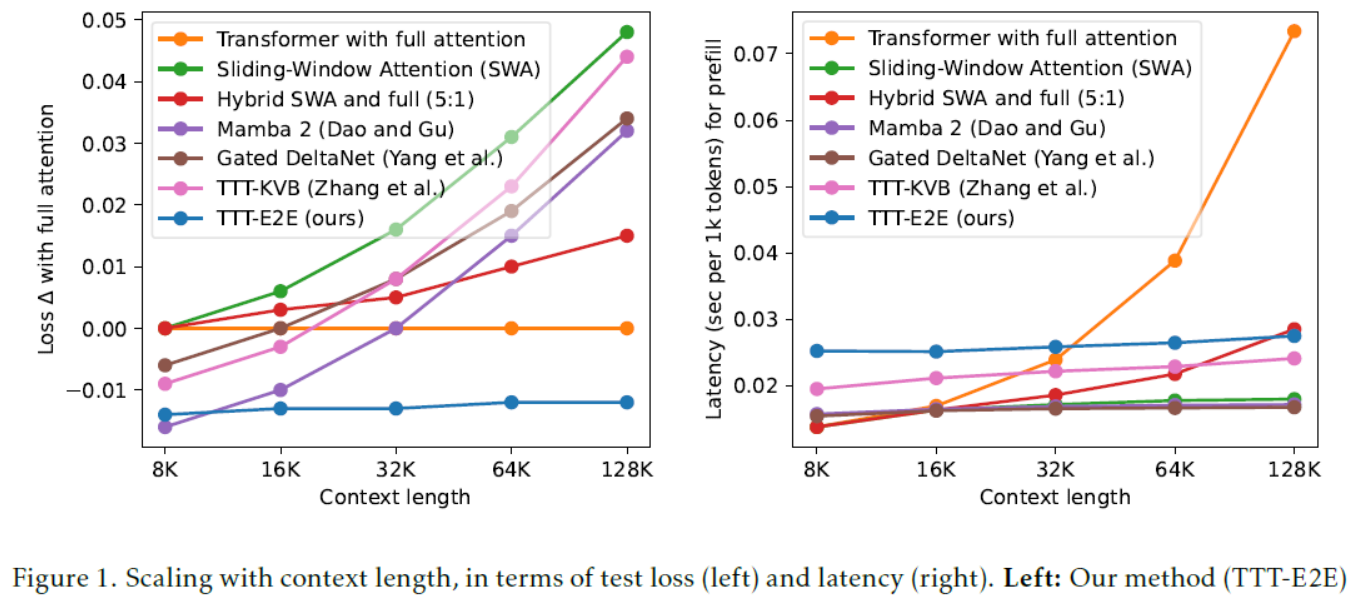
[Figure 1:Scaling with context length, in terms of test loss (left) and latency (right). Left: Our method (TTT-E2E) turns the worst line (green) into the best (blue) at 128K context length. Loss (↓), the y-value, is computed as (loss of the reported method) − (loss of Transformer with full attention), so loss of full attention itself (orange) is the flat line at y=0. While other methods produce worse loss in longer context, TTT-E2E maintains the same advantage over full attention. All models have 3B parameters and are trained with 164B tokens. Right: Similar to SWA and the RNN baselines, TTT-E2E has constant inference latency regardless of context length, making it 2.7× faster than full attention for 128K context on an H100.图 1：随着上下文长度的变化，测试损失（左）和延迟（右）的变化情况。左：我们的方法（TTT-E2E）将最差的曲线（绿色）在 128K 上下文长度时转变为最佳（蓝色）。损失（↓），即 y 值，计算方式为（所报告方法的损失） - （具有全注意力的 Transformer 的损失），因此全注意力本身的损失（橙色）是 y = 0 的水平线。尽管其他方法在更长的上下文时产生更差的损失，但 TTT-E2E 相对于全注意力仍保持同样的优势。所有模型均具有 30 亿参数，并使用 1640 亿个标记进行训练。右：与 SWA 和 RNN 基线类似，TTT-E2E 的推理延迟与上下文长度无关，因此在 H100 上对于 128K 上下文，其速度比全注意力快 2.7 倍。](#Figure 1:Scaling with context length, in terms of test loss (left) and latency (right). Left: Our method (TTT-E2E) turns the worst line (green) into the best (blue) at 128K context length. Loss (↓), the y-value, is computed as (loss of the reported method) − (loss of Transformer with full attention), so loss of full attention itself (orange) is the flat line at y=0. While other methods produce worse loss in longer context, TTT-E2E maintains the same advantage over full attention. All models have 3B parameters and are trained with 164B tokens. Right: Similar to SWA and the RNN baselines, TTT-E2E has constant inference latency regardless of context length, making it 2.7× faster than full attention for 128K context on an H100.图 1：随着上下文长度的变化，测试损失（左）和延迟（右）的变化情况。左：我们的方法（TTT-E2E）将最差的曲线（绿色）在 128K 上下文长度时转变为最佳（蓝色）。损失（↓），即 y 值，计算方式为（所报告方法的损失） - （具有全注意力的 Transformer 的损失），因此全注意力本身的损失（橙色）是 y = 0 的水平线。尽管其他方法在更长的上下文时产生更差的损失，但 TTT-E2E 相对于全注意力仍保持同样的优势。所有模型均具有 30 亿参数，并使用 1640 亿个标记进行训练。右：与 SWA 和 RNN 基线类似，TTT-E2E 的推理延迟与上下文长度无关，因此在 H100 上对于 128K 上下文，其速度比全注意力快 2.7 倍。)

1、Introduction

[Figure 2:Toy example. Left: Given x1 and x2 as context, we want to predict the unknown x3. Our toy baseline, a Transformer without self-attention (using only the upward arrows), is effectively a bigram since it has no memory of x1. TTT (using all the arrows) first tries to predict x2 from x1 as an exercise: It computes the loss ℓ2 between x2 and the prediction p^2, then takes a gradient step on ℓ2. Now information of x1 is stored in the updated MLPs (blue). Right: Token-level test loss ℓt for various methods in our toy example, as discussed in Subsection 2.2, except for TTT-E2E b=16 discussed in Subsection 2.3. In particular, TTT-E2E b=1 turns the green line (our toy baseline) into the blue line, which performs almost as well as orange (using full attention).图 2：示例。左：给定 x1 和 x2 作为上下文，我们想要预测未知的 x3。我们的示例基线是一个没有自注意力的 Transformer（仅使用向上的箭头），由于它没有 x1 的记忆，所以实际上是一个二元模型。TTT（使用所有箭头）首先尝试从 x1 预测 x2 作为练习：它计算 x2 和预测值 p^2 之间的损失 ℓ2，然后对 ℓ2 进行梯度下降。现在 x1 的信息存储在更新后的 MLP（蓝色）中。右：在我们的示例中，各种方法的标记级测试损失 ℓt，如 2.2 节所述，除了 2.3 节讨论的 TTT-E2E b=16。特别是，TTT-E2E b=1 将绿色线（我们的示例基线）变为蓝色线，其表现几乎与橙色线（使用全注意力）一样好。](#Figure 2:Toy example. Left: Given x1 and x2 as context, we want to predict the unknown x3. Our toy baseline, a Transformer without self-attention (using only the upward arrows), is effectively a bigram since it has no memory of x1. TTT (using all the arrows) first tries to predict x2 from x1 as an exercise: It computes the loss ℓ2 between x2 and the prediction p^2, then takes a gradient step on ℓ2. Now information of x1 is stored in the updated MLPs (blue). Right: Token-level test loss ℓt for various methods in our toy example, as discussed in Subsection 2.2, except for TTT-E2E b=16 discussed in Subsection 2.3. In particular, TTT-E2E b=1 turns the green line (our toy baseline) into the blue line, which performs almost as well as orange (using full attention).图 2：示例。左：给定 x1 和 x2 作为上下文，我们想要预测未知的 x3。我们的示例基线是一个没有自注意力的 Transformer（仅使用向上的箭头），由于它没有 x1 的记忆，所以实际上是一个二元模型。TTT（使用所有箭头）首先尝试从 x1 预测 x2 作为练习：它计算 x2 和预测值 p^2 之间的损失 ℓ2，然后对 ℓ2 进行梯度下降。现在 x1 的信息存储在更新后的 MLP（蓝色）中。右：在我们的示例中，各种方法的标记级测试损失 ℓt，如 2.2 节所述，除了 2.3 节讨论的 TTT-E2E b=16。特别是，TTT-E2E b=1 将绿色线（我们的示例基线）变为蓝色线，其表现几乎与橙色线（使用全注意力）一样好。)

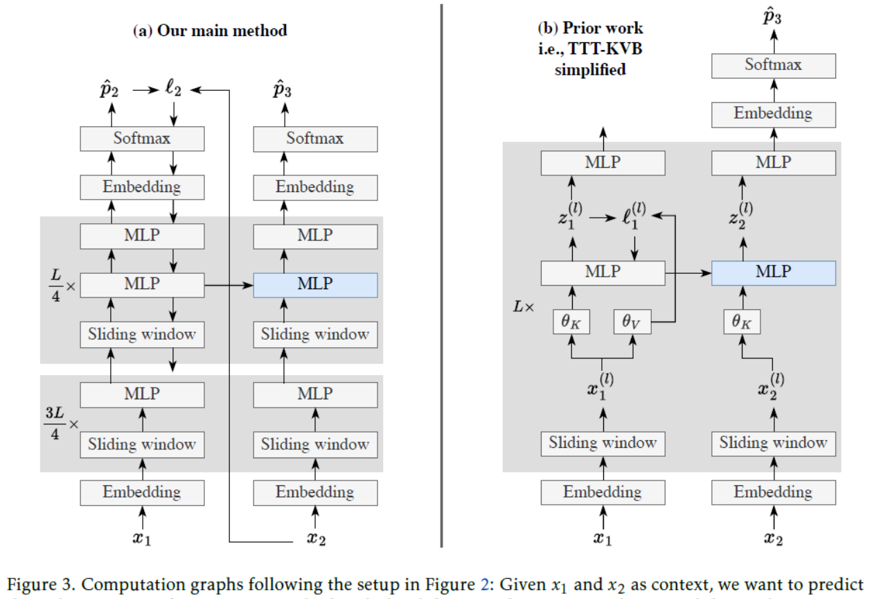
[Figure 3: Computation graphs following the setup in Figure 2: Given x1 and x2 as context, we want to predict the unknown x3. Left: Our main method with the sliding-window attention layers and the implementation details discussed in Subsection 2.3. For ease of notation, our illustration uses online gradient descent (b=1). The lowest downward arrow is disconnected to the MLP below, since gradients pass through the last L/4 blocks but not further down. Right: The first step of our alternative derivation in Subsection 2.4: a simplified version of TTT-KVB in prior work.图 3：遵循图 2 中设置的计算图：给定 x1 和 x2 作为上下文，我们想要预测未知的 x3。左：我们的主要方法，带有滑动窗口注意力层以及在 2.3 小节中讨论的实现细节。为便于表示，我们的示例使用在线梯度下降（b=1）。最下方的向下箭头未与下方的多层感知机相连，因为梯度仅通过最后的 L/4 个块传递，而不会进一步向下传递。右：2.4 小节中我们替代推导的第一步：先前工作中 TTT-KVB 的简化版本。](#Figure 3: Computation graphs following the setup in Figure 2: Given x1 and x2 as context, we want to predict the unknown x3. Left: Our main method with the sliding-window attention layers and the implementation details discussed in Subsection 2.3. For ease of notation, our illustration uses online gradient descent (b=1). The lowest downward arrow is disconnected to the MLP below, since gradients pass through the last L/4 blocks but not further down. Right: The first step of our alternative derivation in Subsection 2.4: a simplified version of TTT-KVB in prior work.图 3：遵循图 2 中设置的计算图：给定 x1 和 x2 作为上下文，我们想要预测未知的 x3。左：我们的主要方法，带有滑动窗口注意力层以及在 2.3 小节中讨论的实现细节。为便于表示，我们的示例使用在线梯度下降（b=1）。最下方的向下箭头未与下方的多层感知机相连，因为梯度仅通过最后的 L/4 个块传递，而不会进一步向下传递。右：2.4 小节中我们替代推导的第一步：先前工作中 TTT-KVB 的简化版本。)

[6 Conclusion](#6 Conclusion)

《End-to-End Test-Time Training for Long Context》翻译与解读

|------------|--------------------------------------------------------------------------------------------------------------|
| 地址 | 论文地址：https://arxiv.org/abs/2512.23675 |
| 时间 | 2025年12月29日 2025年12月31日 |
| 作者 | Astera研究所英伟达斯坦福大学加州大学伯克利分校加州大学圣地亚哥分校 |

Abstract

Figure 1 :Scaling with context length, in terms of test loss (left) and latency (right). Left: Our method (TTT-E2E) turns the worst line (green) into the best (blue) at 128K context length. Loss (↓), the y-value, is computed as (loss of the reported method) − (loss of Transformer with full attention), so loss of full attention itself (orange) is the flat line at y=0. While other methods produce worse loss in longer context, TTT-E2E maintains the same advantage over full attention. All models have 3B parameters and are trained with 164B tokens. Right: Similar to SWA and the RNN baselines, TTT-E2E has constant inference latency regardless of context length, making it 2.7× faster than full attention for 128K context on an H100.图 1：随着上下文长度的变化，测试损失（左）和延迟（右）的变化情况。左：我们的方法（TTT-E2E）将最差的曲线（绿色）在 128K 上下文长度时转变为最佳（蓝色）。损失（↓），即 y 值，计算方式为（所报告方法的损失） - （具有全注意力的 Transformer 的损失），因此全注意力本身的损失（橙色）是 y = 0 的水平线。尽管其他方法在更长的上下文时产生更差的损失，但 TTT-E2E 相对于全注意力仍保持同样的优势。所有模型均具有 30 亿参数，并使用 1640 亿个标记进行训练。右：与 SWA 和 RNN 基线类似，TTT-E2E 的推理延迟与上下文长度无关，因此在 H100 上对于 128K 上下文，其速度比全注意力快 2.7 倍。

1、Introduction

|--------------------------------------------------------------------------------------------------------------------------------------------------------------------------------------------------------------------------------------------------------------------------------------------------------------------------------------------------------------------------------------------------------------------------------------------------------------------------------------------------------------------------------------------------------------------------------------------------------------------------------------------------------------------------------------------------------------------------------------------------------------------------------------------------------------------------------------------------------------------------------------------------------------------------------------------------------------------------------------------------------------------------------------------------------------------------------------------------------------------------------------------------------------------------------------------------------------------------------------------------------------------------------------------------------------------------------------------------------------------------------------------------------------------------------------------------------------------------------------------------------------------------------------------------------------------------------------------------------------------------------------------------------------------------------------------------------------------------------------------------------------------------------------------------------------------------------------------------------------------------------------------------------------------------------------------------------------------------------------------------------------------------------------------------------------------------|----------------------------------------------------------------------------------------------------------------------------------------------------------------------------------------------------------------------------------------------------------------------------------------------------------------------------------------------------------------------------------------------------------------------------------------------------------------------------------------------------------------------------------------------------------------------------------------------------------------------------------------------------------------------------------------------------------------------------|
| Humans are able to improve themselves with more experience throughout their lives, despite their imperfect recall of the exact details. Consider your first lecture in machine learning: You might not recall the instructor's first word during the lecture, but the intuition you learned is probably helping you understand this paper, even if that lecture happened years ago. On the other hand, Transformers with self-attention still struggle to efficiently process long context equivalent to years of human experience, in part because they are designed for nearly lossless recall. Self-attention over the full context, also known as full attention, must scan through the keys and values of all previous tokens for every new token. As a consequence, it readily attends to every detail, but its cost per token grows linearly with context length and quickly becomes prohibitive. As an alternative to Transformers, RNNs such as Mamba 2 [32] and Gated DeltaNet [104] have constant cost per token, but become less effective in longer context, as shown in Figure 1. Some modern architectures approximate full attention with a sliding window [1, 107], or stack attention and RNN layers together [91, 11]. However, these techniques are still less effective than full attention in using longer context to achieve better performance in language modeling. How can we design an effective method for language modeling with only constant cost per token?Specifically, how can we achieve better performance in longer context without recalling every detail, as in the opening example? The key mechanism is compression. For example, humans compress a massive amount of experience into their brains, which preserve the important information while leaving out many details. For language models, training with next-token prediction also compresses a massive amount of data into their weights. So what if we just continue training the language model at test time via next-token prediction on the given context? | 尽管人类对具体细节的回忆并不完美，但他们在一生中能够通过不断积累经验来提升自我。想想你第一次听机器学习的讲座：你或许记不起讲师在讲座中的第一句话，但你学到的直觉可能正在帮助你理解这篇论文，即便那次讲座已经过去多年。另一方面，带有自注意力机制的 Transformer 模型在处理相当于人类多年经验的长上下文时仍面临效率难题，部分原因在于它们的设计旨在实现近乎无损的回忆。对于每个新标记，全自注意力（也称为全注意力）都需要扫描所有先前标记的键和值。因此，它能够关注到每一个细节，但其每标记的成本随上下文长度线性增长，很快就会变得难以承受。作为 Transformer 的替代方案，诸如 Mamba 2 [32] 和 Gated DeltaNet [104] 这样的循环神经网络（RNN）每标记的成本是恒定的，但在处理更长的上下文时效果会变差，如图 1 所示。一些现代架构通过滑动窗口来近似实现全注意力机制[1, 107]，或者将注意力机制与 RNN 层堆叠在一起[91, 11]。然而，这些技术在利用更长的上下文来提高语言模型性能方面，仍不如全注意力机制有效。如何设计一种仅需固定成本就能有效进行语言建模的方法？具体来说，在不回忆每个细节的情况下，如何在更长的上下文中实现更好的性能，就像开头的例子那样？关键机制在于压缩。例如，人类将大量的经验压缩到大脑中，保留重要信息，同时舍弃许多细节。对于语言模型来说，通过下个词预测进行训练也会将大量数据压缩到其权重中。那么，如果我们在测试时通过在给定的上下文中进行下个词预测来继续训练语言模型会怎样呢？ |
| This form of Test-Time Training (TTT), similar to an old idea known as dynamic evaluation [72, 60], still has a missing piece: At training time, we were optimizing the model for its loss out of the box, not for its loss after TTT. To resolve this mismatch, we prepare the model's initialization for TTT via meta-learning [38, 79, 58] instead of standard pre-training. Specifically, each training sequence is first treated as if it were a test sequence, so we perform TTT on it in the inner loop. Then we average the loss after TTT over many independent training sequences, and optimize this average w.r.t. the model's initialization for TTT through gradients of gradients in the outer loop [71, 3, 27]. In summary, our method is end-to-end in two ways. Our inner loop directly optimizes the next-token prediction loss at the end of the network, in contrast to prior work on long-context TTT [86, 110]; Subsection 2.4 explains this difference through an alternative derivation of our method. Moreover, our outer loop directly optimizes the final loss after TTT, in contrast to dynamic evaluation [72, 60], as discussed. Our key results are highlighted in Figure 1, with the rest presented in Section 3. The conceptual framework of TTT has a long history with many applications beyond long context, and many forms without meta-learning [85, 12, 45, 2]. Our work is also inspired by the literature on fast weights [38, 79, 77, 49], especially [17] by Clark et al., which shares our high-level approach. Section 4 discusses related work in detail. | 这种测试时训练（TTT）的形式类似于一种旧的理念，即动态评估[72, 60]，但它仍有一个缺失的部分：在训练时，我们优化的是模型的初始损失，而不是经过 TTT 后的损失。为解决这种不匹配问题，我们通过元学习[38, 79, 58]而非标准预训练来为 TTT 准备模型的初始化。具体来说，首先将每个训练序列当作测试序列处理，因此在内循环中对其执行 TTT。然后，我们对许多独立训练序列的 TTT 后损失取平均值，并在外循环中通过梯度的梯度针对 TTT 的模型初始化优化此平均值[71, 3, 27]。总之，我们的方法在两个方面是端到端的。我们的内循环直接优化网络末尾的下一个标记预测损失，这与先前关于长上下文 TTT 的工作[86, 110]不同；第 2.4 节通过另一种推导方式解释了这种差异。此外，我们的外循环直接优化 TTT 后的最终损失，这与动态评估[72, 60]不同，如前所述。我们的关键结果在图 1 中突出显示，其余结果在第 3 节中给出。 TTT 的概念框架有着悠久的历史，其应用远不止长上下文，并且有许多不包含元学习的形式[85, 12, 45, 2]。我们的工作也受到快速权重相关文献[38, 79, 77, 49]的启发，尤其是克拉克等人[17]的工作，其与我们的高层次方法一致。第 4 节详细讨论了相关工作。 |

Figure 2:Toy example. Left: Given x1 and x2 as context, we want to predict the unknown x3. Our toy baseline, a Transformer without self-attention (using only the upward arrows), is effectively a bigram since it has no memory of x1. TTT (using all the arrows) first tries to predict x2 from x1 as an exercise: It computes the loss ℓ2 between x2 and the prediction p^2, then takes a gradient step on ℓ2. Now information of x1 is stored in the updated MLPs (blue). Right: Token-level test loss ℓt for various methods in our toy example, as discussed in Subsection 2.2, except for TTT-E2E b=16 discussed in Subsection 2.3. In particular, TTT-E2E b=1 turns the green line (our toy baseline) into the blue line, which performs almost as well as orange (using full attention).图 2：示例。左：给定 x1 和 x2 作为上下文，我们想要预测未知的 x3。我们的示例基线是一个没有自注意力的 Transformer（仅使用向上的箭头），由于它没有 x1 的记忆，所以实际上是一个二元模型。TTT（使用所有箭头）首先尝试从 x1 预测 x2 作为练习：它计算 x2 和预测值 p^2 之间的损失 ℓ2，然后对 ℓ2 进行梯度下降。现在 x1 的信息存储在更新后的 MLP（蓝色）中。右：在我们的示例中，各种方法的标记级测试损失 ℓt，如 2.2 节所述，除了 2.3 节讨论的 TTT-E2E b=16。特别是，TTT-E2E b=1 将绿色线（我们的示例基线）变为蓝色线，其表现几乎与橙色线（使用全注意力）一样好。

Figure 3: Computation graphs following the setup in Figure 2: Given x1 and x2 as context, we want to predict the unknown x3. Left: Our main method with the sliding-window attention layers and the implementation details discussed in Subsection 2.3. For ease of notation, our illustration uses online gradient descent (b=1). The lowest downward arrow is disconnected to the MLP below, since gradients pass through the last L/4 blocks but not further down. Right: The first step of our alternative derivation in Subsection 2.4: a simplified version of TTT-KVB in prior work.图 3：遵循图 2 中设置的计算图：给定 x1 和 x2 作为上下文，我们想要预测未知的 x3。左：我们的主要方法，带有滑动窗口注意力层以及在 2.3 小节中讨论的实现细节。为便于表示，我们的示例使用在线梯度下降（b=1）。最下方的向下箭头未与下方的多层感知机相连，因为梯度仅通过最后的 L/4 个块传递，而不会进一步向下传递。右：2.4 小节中我们替代推导的第一步：先前工作中 TTT-KVB 的简化版本。