今天我们来理解一下LQR控制,以及通过一个基本的轨迹跟踪进行具体的描述.并且为了加深理解,我们需要对LQR和MPC的区别进行详细的剖析.
LQR 是一种现代控制理论中的最优控制方法。它的核心思想不是"简单地把误差消除",而是"以最小的代价把误差消除"。
1. 数学本质
LQR 试图在一个线性系统 x˙=Ax+Bu\dot{x} = Ax + Bux˙=Ax+Bu 中,寻找一个控制律 u=−Kxu = -Kxu=−Kx,使得以下的代价函数 (Cost Function) JJJ 最小:
J=∫0∞(xTQx+uTRu)dtJ = \int_{0}^{\infty} (x^T Q x + u^T R u) dtJ=∫0∞(xTQx+uTRu)dt
xxx (State Error): 状态偏差(如:横向误差、航向误差)。
uuu (Control Input): 控制输入(如:转角、加速度)。
QQQ (State Cost Matrix): 状态权重矩阵。如果 QQQ 很大:表示你非常在乎误差(必须要准),控制会很激进。
RRR (Input Cost Matrix): 输入权重矩阵。如果 RRR 很大:表示你非常在乎能量消耗或舒适度(方向盘不能乱打),控制会很柔和。
2. LQR 的工作流程
-
线性化 (Linearization): 车辆运动学模型是非线性的(因为有 sin(θ),cos(θ)sin(\theta), cos(\theta)sin(θ),cos(θ))。LQR 只能处理线性系统,所以在每个时间步,你都在参考点附近计算了雅可比矩阵 AAA 和 BBB 。
-
求解黎卡提方程 (Riccati Equation): 为了找到最优的 KKK,必须求解代数黎卡提方程 (DARE)。
-
反馈控制: 计算出增益 KKK 后,控制量即为 u=−K×erroru = -K \times erroru=−K×error。
3. 物理直觉与优缺点优点:
优点
- 算得快: 求解 KKK 矩阵非常快,适合实时嵌入式系统。
- 稳定性: 对于线性系统,LQR 保证闭环系统是稳定的。
- 参数物理意义明确: 调 QQQ 就是调精度,调 RRR 就是调平顺性。
缺点
- 无约束处理能力: 这是 LQR 最大的痛点。比如车辆最大转角是 35度,LQR 计算出的最优解可能是 50度。必须在代码中手动 np.clip,但这已经不是"最优"了(被截断了)。
- 不看未来: 标准 LQR 假设是无限时间视界,它主要看当前误差来反应,缺乏对"未来已知弯道"的提前规划能力。
实验一.不同R对控制效果的影响
python
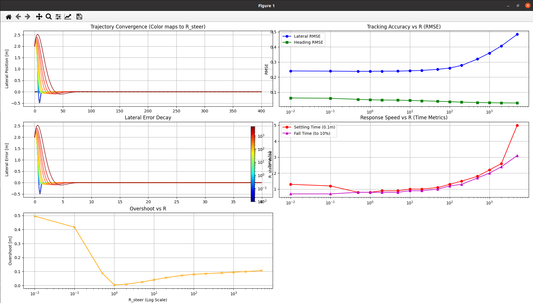
# R值越小:控制越激进,误差收敛越快,但对执行机构(电机、转向机)要求高,且容易导致乘客不适或系统震荡。
# R值越大:控制越平滑,能量消耗越低,但跟踪误差消除得很慢,在这个场景下表现为"反应迟钝"。
# 全指标计算: 增加了专门的函数来计算超调量(Overshoot)、上升/下降时间(Rise/Fall Time)、调节时间(Settling Time)以及各项 RMSE。
import numpy as np
import matplotlib.pyplot as plt
import matplotlib.cm as cm
import matplotlib.colors as mcolors
import scipy.linalg as la
import pandas as pd

# ================= 1. 系统配置 =================
L = 3.8             # 轴距 (m)
DT = 0.1            # 采样时间 (s)
SIM_TIME = 40.0     # 仿真时长 (s)
TARGET_SPEED = 10.0 # 目标速度 (m/s)

# 初始状态
X0, Y0, V0, THETA0 = 0.0, 2.0, 10.0, 0.2

# 权重矩阵
Q = np.diag([0.0, 10.0, 5.0, 10.0]) # [x, y, v, theta]
R_ACC_FIXED = 1.0

# 定义 R_steer 扫描范围 (包含对数分布的密集采样)
R_TEST_VALUES = [0.01, 0.1, 0.5, 1.0, 2.0, 5.0, 10.0, 20.0, 50.0,
                 100.0, 200.0, 500.0, 1000.0, 2000.0, 5000.0]

# ================= 2. 核心算法 =================

def normalize_angle(angle):
    while angle > np.pi: angle -= 2.0 * np.pi
    while angle < -np.pi: angle += 2.0 * np.pi
    return angle

def solve_lqr(A, B, Q, R):
    try:
        P = la.solve_discrete_are(A, B, Q, R)
        K = la.inv(R + B.T @ P @ B) @ (B.T @ P @ A)
    except:
        return np.zeros((2, 4))
    return K

def model_step(state, u):
    x, y, v, theta = state
    a, delta = u
    delta = np.clip(delta, -np.radians(35), np.radians(35)) # 物理约束

    x_new = x + v * np.cos(theta) * DT
    y_new = y + v * np.sin(theta) * DT
    v_new = v + a * DT
    theta_new = theta + v / L * np.tan(delta) * DT

    return np.array([x_new, y_new, v_new, normalize_angle(theta_new)])

def get_linearized_matrices(v_ref, phi_ref, delta_ref=0.0):
    A = np.eye(4)
    A[0, 2] = np.cos(phi_ref) * DT
    A[0, 3] = -v_ref * np.sin(phi_ref) * DT
    A[1, 2] = np.sin(phi_ref) * DT
    A[1, 3] = v_ref * np.cos(phi_ref) * DT
    A[3, 2] = np.tan(delta_ref) / L * DT

    B = np.zeros((4, 2))
    B[2, 0] = DT
    B[3, 1] = v_ref / (L * np.cos(delta_ref)**2) * DT
    return A, B

# ================= 3. 指标计算工具 =================

def calculate_metrics(t_arr, y_arr, v_arr, theta_arr, r_val):
    """
    计算控制性能指标
    """
    y_arr = np.array(y_arr)
    theta_arr = np.array(theta_arr)
    v_arr = np.array(v_arr)

    # 1. RMSE (均方根误差)
    rmse_lat = np.sqrt(np.mean(y_arr**2))
    rmse_head = np.sqrt(np.mean(theta_arr**2))
    rmse_spd = np.sqrt(np.mean((v_arr - TARGET_SPEED)**2))

    # 2. Settling Time (调节时间): 进入并保持在 +/- 0.1m 误差带的时间
    # 倒序查找第一个不满足条件的索引
    abs_y = np.abs(y_arr)
    threshold = 0.1
    outside_band = np.where(abs_y > threshold)[0]
    if len(outside_band) > 0:
        settle_idx = outside_band[-1] + 1
        if settle_idx < len(t_arr):
            settling_time = t_arr[settle_idx]
        else:
            settling_time = np.nan # 未收敛
    else:
        settling_time = 0.0

    # 3. Rise Time (此处定义为 Fall Time): 首次从初始误差下降到 10% 的时间
    target_10_percent = np.abs(Y0) * 0.1
    reached_10 = np.where(abs_y <= target_10_percent)[0]
    if len(reached_10) > 0:
        rise_time = t_arr[reached_10[0]]
    else:
        rise_time = np.nan

    # 4. Overshoot (超调量):
    # 既然目标是0,初始是正,看有没有变成负数。取最大的负偏离绝对值。
    # 定义超调量为:最大反向偏差的绝对值
    min_y = np.min(y_arr)
    overshoot = abs(min_y) if min_y < 0 else 0.0

    return {
        "R_steer": r_val,
        "RMSE_Lat": rmse_lat,
        "RMSE_Head": rmse_head,
        "RMSE_Spd": rmse_spd,
        "Settling_Time": settling_time,
        "Rise_Time": rise_time,
        "Overshoot": overshoot
    }

# ================= 4. 仿真与统计 =================

results_list = []
metrics_list = []

for r_val in R_TEST_VALUES:
    R = np.diag([R_ACC_FIXED, r_val])
    state = np.array([X0, Y0, V0, THETA0])

    history = {'t': [], 'x': [], 'y': [], 'v': [], 'theta': [], 'steer': []}

    for t in np.arange(0, SIM_TIME, DT):
        ref = np.array([state[0] + TARGET_SPEED*DT, 0.0, TARGET_SPEED, 0.0])
        error = state - ref
        error[3] = normalize_angle(error[3])

        A, B = get_linearized_matrices(ref[2], ref[3])
        K = solve_lqr(A, B, Q, R)
        u = -K @ error

        history['t'].append(t)
        history['x'].append(state[0])
        history['y'].append(state[1])
        history['v'].append(state[2])
        history['theta'].append(state[3])
        history['steer'].append(u[1])

        state = model_step(state, u)

    # 存储轨迹数据
    history['r_val'] = r_val
    results_list.append(history)

    # 计算指标
    metrics = calculate_metrics(history['t'], history['y'], history['v'], history['theta'], r_val)
    metrics_list.append(metrics)

# 生成 Pandas 表格
df_metrics = pd.DataFrame(metrics_list)

# ================= 5. 可视化 =================

fig = plt.figure(figsize=(18, 12))
gs = fig.add_gridspec(3, 2)

# Colormap
norm = mcolors.LogNorm(vmin=min(R_TEST_VALUES), vmax=max(R_TEST_VALUES))
cmap = cm.jet

# 1. 轨迹图 (XY)
ax1 = fig.add_subplot(gs[0, 0])
ax1.plot([0, 400], [0, 0], 'k--', lw=2, label="Reference")
for res in results_list:
    color = cmap(norm(res['r_val']))
    ax1.plot(res['x'], res['y'], color=color, lw=1.5, alpha=0.8)
ax1.set_title("Trajectory Convergence (Color maps to R_steer)")
ax1.set_ylabel("Lateral Position [m]")
ax1.grid(True)

# 2. 横向误差 (Time vs Y)
ax2 = fig.add_subplot(gs[1, 0])
for res in results_list:
    color = cmap(norm(res['r_val']))
    ax2.plot(res['t'], res['y'], color=color, lw=1.5, alpha=0.8)
ax2.set_title("Lateral Error Decay")
ax2.set_ylabel("Lateral Error [m]")
ax2.grid(True)

# 3. 统计指标趋势分析 (Trade-off Visualization)
# RMSE vs R
ax3 = fig.add_subplot(gs[0, 1])
ax3.semilogx(df_metrics['R_steer'], df_metrics['RMSE_Lat'], 'b-o', label='Lateral RMSE')
ax3.semilogx(df_metrics['R_steer'], df_metrics['RMSE_Head'], 'g-s', label='Heading RMSE')
ax3.set_title("Tracking Accuracy vs R (RMSE)")
ax3.set_ylabel("RMSE")
ax3.legend()
ax3.grid(True)

# Time Metrics vs R
ax4 = fig.add_subplot(gs[1, 1])
ax4.semilogx(df_metrics['R_steer'], df_metrics['Settling_Time'], 'r-o', label='Settling Time (0.1m)')
ax4.semilogx(df_metrics['R_steer'], df_metrics['Rise_Time'], 'm-^', label='Fall Time (to 10%)')
ax4.set_title("Response Speed vs R (Time Metrics)")
ax4.set_ylabel("Time [s]")
ax4.legend()
ax4.grid(True)

# Overshoot vs R
ax5 = fig.add_subplot(gs[2, 0])
ax5.semilogx(df_metrics['R_steer'], df_metrics['Overshoot'], 'k-x', color='orange')
ax5.set_title("Overshoot vs R")
ax5.set_xlabel("R_steer (Log Scale)")
ax5.set_ylabel("Overshoot [m]")
ax5.grid(True)

# Colorbar for reference
sm = cm.ScalarMappable(cmap=cmap, norm=norm)
sm.set_array([])
cbar = plt.colorbar(sm, ax=[ax1, ax2, ax5], location='right', fraction=0.02)
cbar.set_label('R_steer Value')

# 打印统计报表
print("===== LQR 参数扫描性能统计表 =====")
# 格式化打印
pd.set_option('display.float_format', lambda x: '%.4f' % x)
print(df_metrics[['R_steer', 'RMSE_Lat', 'Overshoot', 'Rise_Time', 'Settling_Time']])

plt.tight_layout()
plt.show()
从相关误差上来分析,我们可以看到越小的R所需要的控制是越长时间的,对于误差也就是越来越不在意,所以误差是在变大的.
LQR 与 MPC (Model Predictive Control) 的区别
LQR 像是一个经验丰富的老司机,凭直觉(增益 KKK)瞬间做出反应,但他不管物理极限,需要你帮他踩刹车限制。
MPC 像是一个下棋大师,每走一步都要推演未来 N 步的最优解,并且严格遵守所有规则(约束),但他思考的时间比较长。
- 数学形式的深度对比
假设我们需要控制一个离散线性系统:xk+1=Axk+Bukx_{k+1} = A x_k + B u_kxk+1=Axk+Buk(1) LQR 的数学表达:无拘无束的理想主义者
LQR 试图寻找控制律 uk=−Kxku_k = -K x_kuk=−Kxk,使得无限时间内的代价最小。优化目标 (Objective):JLQR=∑k=0∞(xkTQxk+ukTRuk)J_{LQR} = \sum_{k=0}^{\infty} (x_k^T Q x_k + u_k^T R u_k)JLQR=k=0∑∞(xkTQxk+ukTRuk)约束条件 (Subject to):
1.系统动力学: xk+1=Axk+Bukx_{k+1} = A x_k + B u_kxk+1=Axk+Buk
2.物理约束: 无 (None) ←\leftarrow← 这是 LQR 的死穴
数学本质:因为是对无限时间积分且无约束,这个问题可以通过求解代数黎卡提方程 (DARE) 得到一个完美的解析解 PPP。
P=ATPA−ATPB(R+BTPB)−1BTPA+QP = A^T P A - A^T P B (R + B^T P B)^{-1} B^T P A + QP=ATPA−ATPB(R+BTPB)−1BTPA+Q
最终得到的增益 KKK 是一个常数矩阵。
(2) MPC 的数学表达:戴着镣铐的精算师
MPC 试图在每个时刻 ttt,寻找未来 NNN 步的控制序列,使得有限时间内的代价最小,且严格满足约束。
优化目标 (Objective):
JMPC=xNTPxN⏟终端代价+∑k=0N−1(xkTQxk+ukTRuk)J_{MPC} = \underbrace{x_N^T P x_N}{\text{终端代价}} + \sum{k=0}^{N-1} (x_k^T Q x_k + u_k^T R u_k)JMPC=终端代价 xNTPxN+k=0∑N−1(xkTQxk+ukTRuk)
约束条件 (Subject to):
1.系统动力学: xk+1=Axk+Bukx_{k+1} = A x_k + B u_kxk+1=Axk+Buk初始状态: x0=x(t)x_0 = x(t)x0=x(t) (当前传感器测得的状态)
2.输入约束: umin≤uk≤umaxu_{min} \le u_k \le u_{max}umin≤uk≤umax (例如:方向盘最大转角 ±35∘\pm 35^\circ±35∘) ←\leftarrow← LQR 做不到
3.状态约束: xmin≤xk≤xmaxx_{min} \le x_k \le x_{max}xmin≤xk≤xmax (例如:位置不能超出车道线)
4.数学本质:这就变成了一个二次规划 (Quadratic Programming, QP) 问题:min12UTHU+fTUs.t.GU≤W\min \frac{1}{2} U^T H U + f^T U \quad \text{s.t.} \quad G U \le Wmin21UTHU+fTUs.t.GU≤W
-
这不是解方程,这是在多维空间里找极值点。
-
因为有不等式约束 (GU≤WG U \le WGU≤W),它没有解析解(写不出公式),只能用数值迭代法(如 Interior Point Method)硬算。
-
引入 cvxpy 库来求解 MPC 的凸优化问题(这是 Python 中最标准的 MPC 实现方式)。
-
设置了一个较硬的物理约束(方向盘最大转角),你会看到 MPC 会贴着约束走,而 LQR 会被截断。
注意: 运行此代码需要安装 cvxpy:
pip install cvxpy
实验二
python
import numpy as np
import matplotlib.pyplot as plt
import scipy.linalg as la
import cvxpy as cp
import math

# ================= 1. 系统参数 =================
L = 3.8             # 轴距
DT = 0.1            # 采样时间
SIM_TIME = 20.0     # 仿真时长
TARGET_SPEED = 10.0 # 目标速度

# 初始状态 [x, y, v, theta]
# 特意设置一个较大的横向误差,逼迫控制器做出剧烈动作
X0, Y0, V0, THETA0 = 0.0, 3.0, 10.0, 0.0

# 物理约束
MAX_STEER = np.radians(20.0)  # 限制最大转角 20度 (0.35 rad)
MAX_ACCEL = 2.0

# ================= 2. LQR 工具 =================
def solve_lqr(A, B, Q, R):
    P = la.solve_discrete_are(A, B, Q, R)
    K = la.inv(R + B.T @ P @ B) @ (B.T @ P @ A)
    return K

def get_linearized_model(v, phi, delta=0.0):
    A = np.eye(4)
    A[0, 2] = np.cos(phi) * DT
    A[0, 3] = -v * np.sin(phi) * DT
    A[1, 2] = np.sin(phi) * DT
    A[1, 3] = v * np.cos(phi) * DT
    A[3, 2] = np.tan(delta) / L * DT

    B = np.zeros((4, 2))
    B[2, 0] = DT
    B[3, 1] = v / (L * np.cos(delta)**2) * DT
    return A, B

def normalize_angle(angle):
    while angle > np.pi: angle -= 2.0 * np.pi
    while angle < -np.pi: angle += 2.0 * np.pi
    return angle

def update_state(state, a, delta):
    x, y, v, theta = state
    # 强制物理约束 (模拟真实车辆物理限制)
    delta = np.clip(delta, -MAX_STEER, MAX_STEER)
    a = np.clip(a, -MAX_ACCEL, MAX_ACCEL)

    x_new = x + v * np.cos(theta) * DT
    y_new = y + v * np.sin(theta) * DT
    v_new = v + a * DT
    theta_new = theta + v / L * np.tan(delta) * DT
    return np.array([x_new, y_new, v_new, normalize_angle(theta_new)])

# ================= 3. MPC 求解器 (使用 CVXPY) =================
class MPCController:
    def __init__(self, horizon=15):
        self.H = horizon
        self.Q = np.diag([2.0, 10.0, 5.0, 10.0]) # 权重
        self.R = np.diag([1.0, 5.0])             # 输入权重
        self.Rd = np.diag([1.0, 50.0])           # 输入变化率权重 (平滑)

    def solve(self, curr_state, ref_state_traj):
        # 凸优化变量
        x = cp.Variable((4, self.H + 1))
        u = cp.Variable((2, self.H))

        cost = 0
        constraints = []

        # 线性化点 (简化:围绕参考轨迹线性化,或者围绕当前点)
        # 这里为了展示 MPC 威力,使用参考轨迹的线性化模型 (Time-Varying)
        # 简单起见,假设参考轨迹是直的,A, B 恒定
        v_ref = TARGET_SPEED
        phi_ref = 0.0
        A_lin, B_lin = get_linearized_model(v_ref, phi_ref)

        constraints.append(x[:, 0] == curr_state)

        for k in range(self.H):
            # 1. 代价函数: 状态误差 + 输入代价 + 输入平滑度
            state_err = x[:, k] - ref_state_traj[:, k]
            cost += cp.quad_form(state_err, self.Q)
            cost += cp.quad_form(u[:, k], self.R)

            if k > 0:
                cost += cp.quad_form(u[:, k] - u[:, k-1], self.Rd)

            # 2. 动力学约束: x(k+1) = Ax(k) + Bu(k)
            constraints.append(x[:, k+1] == A_lin @ x[:, k] + B_lin @ u[:, k])

            # 3. 硬物理约束 (LQR 做不到的核心点)
            constraints.append(cp.abs(u[0, k]) <= MAX_ACCEL)
            constraints.append(cp.abs(u[1, k]) <= MAX_STEER) # 限制转角

        prob = cp.Problem(cp.Minimize(cost), constraints)
        prob.solve(solver=cp.OSQP, verbose=False) # OSQP 是常用的嵌入式求解器

        if prob.status == cp.OPTIMAL or prob.status == cp.OPTIMAL_INACCURATE:
            return u[:, 0].value, x[:, :].value
        else:
            return np.zeros(2), None

# ================= 4. 主循环对比 =================

# 共享参数
Q_lqr = np.diag([2.0, 10.0, 5.0, 10.0])
R_lqr = np.diag([1.0, 5.0])

# 初始化
state_lqr = np.array([X0, Y0, V0, THETA0])
state_mpc = np.array([X0, Y0, V0, THETA0])

mpc = MPCController(horizon=15) # 预测未来 1.5秒

history = {
    'lqr': {'x': [], 'y': [], 'steer': [], 'calc_steer': []},
    'mpc': {'x': [], 'y': [], 'steer': [], 'calc_steer': []},
    'ref': {'x': [], 'y': []}
}

print("开始仿真: LQR vs MPC...")
for t in np.arange(0, SIM_TIME, DT):
    # --- 参考轨迹生成 (直线) ---
    # LQR 只看当前参考点
    ref_now = np.array([state_lqr[0] + TARGET_SPEED*DT, 0.0, TARGET_SPEED, 0.0])

    # MPC 需要未来 H 步的参考点
    ref_traj_mpc = np.zeros((4, mpc.H + 1))
    for k in range(mpc.H + 1):
        ref_traj_mpc[0, k] = state_mpc[0] + TARGET_SPEED * (k * DT) # X 推进
        ref_traj_mpc[1, k] = 0.0                                    # Y 目标
        ref_traj_mpc[2, k] = TARGET_SPEED                           # V 目标
        ref_traj_mpc[3, k] = 0.0                                    # Theta 目标

    # --- 1. LQR Control ---
    A, B = get_linearized_model(ref_now[2], ref_now[3])
    K = solve_lqr(A, B, Q_lqr, R_lqr)

    error_lqr = state_lqr - ref_now
    error_lqr[3] = normalize_angle(error_lqr[3])

    u_lqr = -K @ error_lqr
    # LQR 计算出的原始值 (可能很大)
    lqr_calc_steer = u_lqr[1]

    # 模拟物理环境并更新状态 (这里会发生物理截断)
    state_lqr = update_state(state_lqr, u_lqr[0], u_lqr[1])

    # --- 2. MPC Control ---
    u_mpc, _ = mpc.solve(state_mpc, ref_traj_mpc)
    mpc_calc_steer = u_mpc[1] # MPC 计算出的值已经满足约束

    state_mpc = update_state(state_mpc, u_mpc[0], u_mpc[1])

    # --- 记录数据 ---
    history['ref']['x'].append(ref_now[0])
    history['ref']['y'].append(ref_now[1])

    history['lqr']['x'].append(state_lqr[0])
    history['lqr']['y'].append(state_lqr[1])
    history['lqr']['steer'].append(state_lqr[3]) # 其实记录的是 theta,为了对齐方便看
    history['lqr']['calc_steer'].append(lqr_calc_steer)

    history['mpc']['x'].append(state_mpc[0])
    history['mpc']['y'].append(state_mpc[1])
    history['mpc']['calc_steer'].append(mpc_calc_steer)

# ================= 5. 绘图对比 =================
plt.figure(figsize=(14, 10))

# 1. 轨迹对比
plt.subplot(2, 1, 1)
plt.plot(history['ref']['x'], history['ref']['y'], 'k--', label='Reference', alpha=0.5)
plt.plot(history['lqr']['x'], history['lqr']['y'], 'b-', linewidth=2, label='LQR Trajectory')
plt.plot(history['mpc']['x'], history['mpc']['y'], 'r-', linewidth=2, label='MPC Trajectory')
plt.title(f'Trajectory Comparison (Initial Y Error = {Y0}m)')
plt.ylabel('Lateral Position [m]')
plt.legend()
plt.grid(True)

# 2. 控制输入 (方向盘转角) 对比
plt.subplot(2, 1, 2)
# 绘制约束线
plt.axhline(y=MAX_STEER, color='k', linestyle=':', label='Physical Limit')
plt.axhline(y=-MAX_STEER, color='k', linestyle=':')

# LQR 计算出的原始输入 (虚线) vs 实际生效输入 (实线效果隐含)
plt.plot(history['lqr']['calc_steer'], 'b--', label='LQR Calculated (Raw)')
plt.plot(np.clip(history['lqr']['calc_steer'], -MAX_STEER, MAX_STEER), 'b-', alpha=0.3, label='LQR Clamped (Actual)')

# MPC 计算出的输入
plt.plot(history['mpc']['calc_steer'], 'r-', linewidth=2, label='MPC Calculated (Constraint Aware)')

plt.title('Steering Control Input Comparison')
plt.ylabel('Steering Angle [rad]')
plt.xlabel('Time Step')
plt.legend()
plt.grid(True)

plt.tight_layout()
plt.show()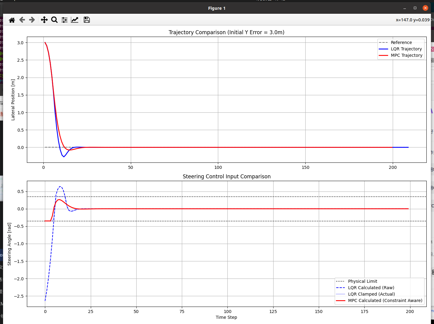
轨迹图 (上图):
LQR: 你会发现 LQR 的轨迹可能会有较大的超调(Overshoot)。因为 LQR 在初始误差很大时,计算出了一个巨大的转角(比如 50 度),但物理只能转 20 度。这导致 LQR 以为自己能很快归位,实际上车辆转不过来,导致收敛变慢甚至震荡。
MPC: MPC 的轨迹通常更平滑,且没有过度超调。因为它在计算第一步时,就已经知道"我最大只能转 20 度,在这个限制下,我大概需要 15 步才能慢慢切回跑道"。
控制输入图 (下图):
LQR Raw (蓝色虚线): 在开始阶段,LQR 计算出的值远远超过了黑色的虚线(物理极限)。这意味着"计算出的最优"在现实中是"不可执行的"。
MPC (红色实线): MPC 的曲线会非常漂亮地贴着黑色的极限线走(Saturation),直到误差减小后才脱离饱和区。这就是 MPC 显式处理约束的能力------它知道边界在哪里,并利用边界跑出最优解。