TensorFlow学习系列03 | 实现天气识别

🍨 本文为 🔗365天深度学习训练营中的学习记录博客
🍖 原作者： K同学啊

一、前置知识

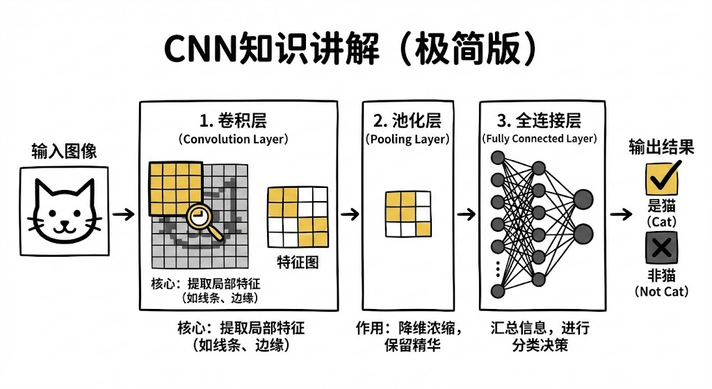
1、CNN知识扫盲

二、代码实现

1、准备工作

1.1.设置GPU

复制代码

import tensorflow as tf
gpus = tf.config.list_physical_devices("GPU")

if gpus:
    gpu0 = gpus[0] #如果有多个GPU，仅使用第0个GPU
    tf.config.experimental.set_memory_growth(gpu0, True) #设置GPU显存用量按需使用
    tf.config.set_visible_devices([gpu0],"GPU")
    
print(gpus)

2026-01-22 23:17:24.154547: I tensorflow/core/util/util.cc:169] oneDNN custom operations are on. You may see slightly different numerical results due to floating-point round-off errors from different computation orders. To turn them off, set the environment variable `TF_ENABLE_ONEDNN_OPTS=0`.
[PhysicalDevice(name='/physical_device:GPU:0', device_type='GPU')]

1.2.导入数据

复制代码

import os,PIL,pathlib
import matplotlib.pyplot as plt
import numpy             as np
from tensorflow          import keras
from tensorflow.keras    import layers,models

# 查看当前工作路径（确认路径是否正确）
print("当前工作路径：", os.getcwd())

# 定义数据目录（建议用绝对路径更稳妥，相对路径依赖当前工作路径）
data_dir = './data/day5_weather_photos/'
data_dir = pathlib.Path(data_dir)

# 获取数据目录下的所有子路径（文件夹或文件）
data_paths = list(data_dir.glob('*'))

# 提取每个子路径的名称（即类别名，自动适配系统分隔符）
classeNames = [path.name for path in data_paths]
classeNames

当前工作路径： /root/autodl-tmp/TensorFlow2

['cloudy', 'rain', 'shine', 'sunrise']

1.3.查看数据

复制代码

image_count = len(list(data_dir.glob('*/*.jpg')))

print("图片总数为：",image_count)

图片总数为： 1125

1.4.可视化图片

复制代码

roses = list(data_dir.glob('sunrise/*.jpg'))
PIL.Image.open(str(roses[0]))

2、数据预处理

2.1.加载数据

使用image_dataset_from_directory方法将磁盘中的数据加载到tf.data.Dataset中

batch_size = 32
img_height = 180
img_width = 180

#训练集
train_ds = tf.keras.preprocessing.image_dataset_from_directory(
data_dir,
validation_split=0.2,
subset="training",
seed=123,
image_size=(img_height, img_width),
batch_size=batch_size)

Found 1125 files belonging to 4 classes.
Using 900 files for training.

验证集

val_ds = tf.keras.preprocessing.image_dataset_from_directory(
data_dir,
validation_split=0.2,
subset="validation",
seed=123,
image_size=(img_height, img_width),
batch_size=batch_size)

Found 1125 files belonging to 4 classes.
Using 225 files for validation.

class_names = train_ds.class_names
print(class_names)

['cloudy', 'rain', 'shine', 'sunrise']

2.2.可视化数据

复制代码

plt.figure(figsize=(20, 10))

for images, labels in train_ds.take(1):
    for i in range(20):
        ax = plt.subplot(5, 10, i + 1)

        plt.imshow(images[i].numpy().astype("uint8"))
        plt.title(class_names[labels[i]])
        
        plt.axis("off")

2.3.检查数据

Image_batch是形状的张量（32,180,180,3）。这是一批形状180x180x3的32张图片（最后一维指的是彩色通道RGB）。

Label_batch是形状（32，）的张量，这些标签对应32张图片

for image_batch, labels_batch in train_ds:
print(image_batch.shape)
print(labels_batch.shape)
break

(32, 180, 180, 3)
(32,)

2.4.配置数据集

复制代码

AUTOTUNE = tf.data.AUTOTUNE

train_ds = train_ds.cache().shuffle(1000).prefetch(buffer_size=AUTOTUNE)
val_ds = val_ds.cache().prefetch(buffer_size=AUTOTUNE)

3、训练模型

3.1.构建CNN网络

复制代码

num_classes = 4

model = models.Sequential([
    layers.experimental.preprocessing.Rescaling(1./255, input_shape=(img_height, img_width, 3)),
    
    layers.Conv2D(16, (3, 3), activation='relu', input_shape=(img_height, img_width, 3)), # 卷积层1，卷积核3*3  
    layers.AveragePooling2D((2, 2)),               # 池化层1，2*2采样
    layers.Conv2D(32, (3, 3), activation='relu'),  # 卷积层2，卷积核3*3
    layers.AveragePooling2D((2, 2)),               # 池化层2，2*2采样
    layers.Conv2D(64, (3, 3), activation='relu'),  # 卷积层3，卷积核3*3
    layers.Dropout(0.3),                           # 让神经元以一定的概率停止工作，防止过拟合，提高模型的泛化能力。
    
    layers.Flatten(),                       # Flatten层，连接卷积层与全连接层
    layers.Dense(128, activation='relu'),   # 全连接层，特征进一步提取
    layers.Dense(num_classes)               # 输出层，输出预期结果
])

model.summary()  # 打印网络结构

Model: "sequential"
_________________________________________________________________
 Layer (type)                Output Shape              Param #   
=================================================================
 rescaling (Rescaling)       (None, 180, 180, 3)       0         
                                                                 
 conv2d (Conv2D)             (None, 178, 178, 16)      448       
                                                                 
 average_pooling2d (AverageP  (None, 89, 89, 16)       0         
 ooling2D)                                                       
                                                                 
 conv2d_1 (Conv2D)           (None, 87, 87, 32)        4640      
                                                                 
 average_pooling2d_1 (Averag  (None, 43, 43, 32)       0         
 ePooling2D)                                                     
                                                                 
 conv2d_2 (Conv2D)           (None, 41, 41, 64)        18496     
                                                                 
 dropout (Dropout)           (None, 41, 41, 64)        0         
                                                                 
 flatten (Flatten)           (None, 107584)            0         
                                                                 
 dense (Dense)               (None, 128)               13770880  
                                                                 
 dense_1 (Dense)             (None, 4)                 516       
                                                                 
=================================================================
Total params: 13,794,980
Trainable params: 13,794,980
Non-trainable params: 0
_________________________________________________________________

3.2.编译模型

复制代码

# 设置优化器
opt = tf.keras.optimizers.Adam(learning_rate=0.001)

model.compile(optimizer=opt,
              loss=tf.keras.losses.SparseCategoricalCrossentropy(from_logits=True),
              metrics=['accuracy'])

3.3.训练模型

复制代码

epochs = 10

history = model.fit(
  train_ds,
  validation_data=val_ds,
  epochs=epochs
)

Epoch 1/10


2026-01-22 23:33:53.565037: I tensorflow/stream_executor/cuda/cuda_dnn.cc:384] Loaded cuDNN version 8101
2026-01-22 23:33:57.017558: I tensorflow/stream_executor/cuda/cuda_blas.cc:1786] TensorFloat-32 will be used for the matrix multiplication. This will only be logged once.


29/29 [==============================] - 8s 33ms/step - loss: 1.3037 - accuracy: 0.5789 - val_loss: 0.5884 - val_accuracy: 0.7689
Epoch 2/10
29/29 [==============================] - 0s 13ms/step - loss: 0.4996 - accuracy: 0.8111 - val_loss: 0.5592 - val_accuracy: 0.7778
Epoch 3/10
29/29 [==============================] - 0s 12ms/step - loss: 0.4080 - accuracy: 0.8500 - val_loss: 0.5595 - val_accuracy: 0.7911
Epoch 4/10
29/29 [==============================] - 0s 13ms/step - loss: 0.3297 - accuracy: 0.8711 - val_loss: 0.4933 - val_accuracy: 0.8178
Epoch 5/10
29/29 [==============================] - 0s 13ms/step - loss: 0.2496 - accuracy: 0.9067 - val_loss: 0.7107 - val_accuracy: 0.7556
Epoch 6/10
29/29 [==============================] - 0s 13ms/step - loss: 0.2371 - accuracy: 0.9044 - val_loss: 0.4809 - val_accuracy: 0.8178
Epoch 7/10
29/29 [==============================] - 0s 13ms/step - loss: 0.1588 - accuracy: 0.9433 - val_loss: 0.4546 - val_accuracy: 0.8533
Epoch 8/10
29/29 [==============================] - 0s 13ms/step - loss: 0.1706 - accuracy: 0.9367 - val_loss: 0.4848 - val_accuracy: 0.8133
Epoch 9/10
29/29 [==============================] - 0s 14ms/step - loss: 0.1061 - accuracy: 0.9600 - val_loss: 0.7095 - val_accuracy: 0.7689
Epoch 10/10
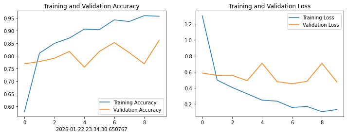
29/29 [==============================] - 0s 13ms/step - loss: 0.1328 - accuracy: 0.9578 - val_loss: 0.4769 - val_accuracy: 0.8622

4、模型评估

复制代码

from datetime import datetime
current_time = datetime.now() # 获取当前时间

acc = history.history['accuracy']
val_acc = history.history['val_accuracy']

loss = history.history['loss']
val_loss = history.history['val_loss']

epochs_range = range(epochs)

plt.figure(figsize=(12, 4))
plt.subplot(1, 2, 1)
plt.plot(epochs_range, acc, label='Training Accuracy')
plt.plot(epochs_range, val_acc, label='Validation Accuracy')
plt.legend(loc='lower right')
plt.title('Training and Validation Accuracy')
plt.xlabel(current_time) # 打卡请带上时间戳，否则代码截图无效

plt.subplot(1, 2, 2)
plt.plot(epochs_range, loss, label='Training Loss')
plt.plot(epochs_range, val_loss, label='Validation Loss')
plt.legend(loc='upper right')
plt.title('Training and Validation Loss')
plt.show()

TensorFlow学习系列03 | 实现天气识别

一、前置知识

1、CNN知识扫盲

二、代码实现

1、准备工作

1.1.设置GPU

1.2.导入数据

1.3.查看数据

1.4.可视化图片

2、数据预处理

2.1.加载数据

验证集

2.2.可视化数据

2.3.检查数据

2.4.配置数据集

3、训练模型

3.1.构建CNN网络

3.2.编译模型

3.3.训练模型

4、模型评估