支持向量机全称是Supported Vector Machine(支持向量机)
即寻找到一个超平面使样本分成两类,并且间隔最大。
• 是一种监督学习算法,主要用于分类,也可用于回归
• 与逻辑回归和决策树等其他分类器相比,SVM 提供了非常高的准确度
优缺点
• 优点:
(1)适合小样本、高纬度数据,比较强泛化能力
(2)可有效地处理高维数据;可使用不同的核函数来适应不同的数据类型
• 缺点:
计算复杂度较高,对于大规模数据的处理可能会存在困难
超平面最大间隔
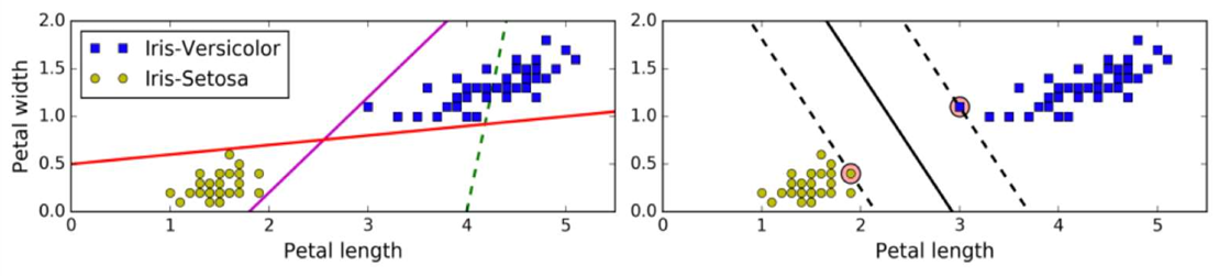
硬间隔Hard Margin
• 如果样本线性可分,在所有样本分类都正确的情况下,寻找最大间隔,这就是硬间隔
• 如果出现异常值、或者样本不能线性可分,此时硬间隔无法实现。
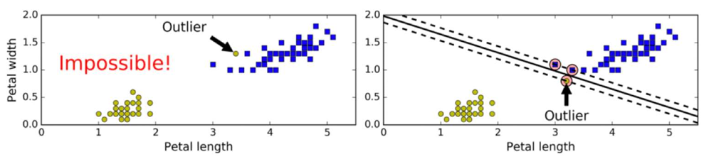
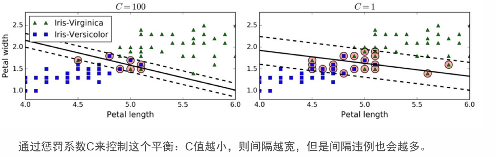
软间隔SoftMargin和惩罚系数
• 允许部分样本,在最大间隔之内,甚至在错误的一边,寻找最大间隔,这就是软间隔
• 目标是尽可能在保持间隔宽阔和限制间隔违例之间找到良好的平衡。
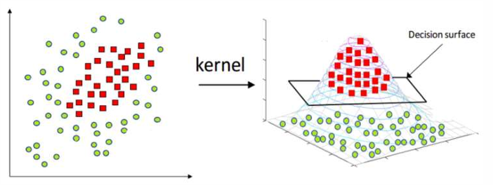
核函数Kernel
核函数将原始输入空间映射到新的特征空间,使得原本线性不可分的样本在核空间可分
使用LinearSVC探索鸢尾花分类 -- API初步使用
plot_util.py
python
import numpy as np
import matplotlib.pyplot as plt


def plot_decision_boundary(model, axis):
    x0, x1 = np.meshgrid(
        np.linspace(axis[0], axis[1], int((axis[1] - axis[0]) * 100)).reshape(-1, 1),
        np.linspace(axis[2], axis[3], int((axis[3] - axis[2]) * 100)).reshape(-1, 1)
    )
    X_new = np.c_[x0.ravel(), x1.ravel()]
    y_predict = model.predict(X_new)
    zz = y_predict.reshape(x0.shape)

    from matplotlib.colors import ListedColormap
    custom_map = ListedColormap(["#EF9A9A", "#FFF59D", "#90CAF9"])

    # plt.contourf(x0,x1,zz,linewidth=5,cmap=custom_map)
    plt.contourf(x0, x1, zz, cmap=custom_map)


def plot_decision_boundary_svc(model, axis):
    x0, x1 = np.meshgrid(
        np.linspace(axis[0], axis[1], int((axis[1] - axis[0]) * 100)).reshape(-1, 1),
        np.linspace(axis[2], axis[3], int((axis[3] - axis[2]) * 100)).reshape(-1, 1)
    )
    X_new = np.c_[x0.ravel(), x1.ravel()]
    y_predict = model.predict(X_new)
    zz = y_predict.reshape(x0.shape)

    from matplotlib.colors import ListedColormap
    custom_map = ListedColormap(["#EF9A9A", "#FFF59D", "#90CAF9"])

    # plt.contourf(x0,x1,zz,linewidth=5,cmap=custom_map)
    plt.contourf(x0, x1, zz, cmap=custom_map)

    w = model.coef_[0]
    b = model.intercept_[0]
    # w0* x0 + w1* x1+ b = 0
    # =>x1 = -w0/w1 * x0 - b/w1
    plot_x = np.linspace(axis[0], axis[1], 200)
    up_y = -w[0] / w[1] * plot_x - b / w[1] + 1 / w[1]
    down_y = -w[0] / w[1] * plot_x - b / w[1] - 1 / w[1]
    up_index = (up_y >= axis[2]) & (up_y <= axis[3])
    down_index = (down_y >= axis[2]) & (down_y <= axis[3])
    plt.plot(plot_x[up_index], up_y[up_index], color="black")
    plt.plot(plot_x[down_index], down_y[down_index], color="black")
python
import numpy as np
import matplotlib.pyplot as plt
from sklearn.svm import LinearSVC
from sklearn.preprocessing import StandardScaler
from sklearn.datasets import load_iris
from plot_util import plot_decision_boundary, plot_decision_boundary_svc
def dm01():
X, y = load_iris(return_X_y=True)
print('X.shape --> ', X.shape)
print('y.shape --> ', y.shape)
X = X[y < 2, :2]
y = y[y < 2]
print('x.shape-->', X.shape)
print('y.shape-->', y.shape)
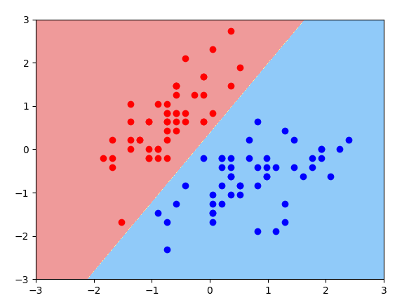
plt.scatter(X[y == 0, 0], X[y == 0, 1], color='red')
plt.scatter(X[y == 1, 0], X[y == 1, 1], color='blue')
plt.show()
transformer = StandardScaler()
X_std = transformer.fit_transform(X)
svc = LinearSVC(dual='auto', C=30)
svc.fit(X_std, y)
plot_decision_boundary(svc, axis=[-3, 3, -3, 3])
plt.scatter(X_std[y == 0, 0], X_std[y == 0, 1], c='red')
plt.scatter(X_std[y == 1, 0], X_std[y == 1, 1], c='blue')
# plt.scatter(X_standard[:, 0], X_standard[:, 1], c=y)
plt.show()
dm01()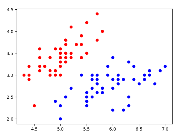
使用LinearSVC探索鸢尾花分类 -- 惩罚参数C对超平面的影响
python
from sklearn.datasets import load_iris
import matplotlib.pyplot as plt
from sklearn.preprocessing import StandardScaler
from sklearn.svm import LinearSVC
from plot_util import plot_decision_boundary_svc


def dm01():
    X, y = load_iris(return_X_y=True)
    print('x.shape -->', X.shape)
    print('y.shape -->', y.shape)

    X = X[y < 2, :2]
    y = y[y < 2]
    print('x.shape-->', X.shape)
    print('y.shape-->', y.shape)

    plt.scatter(X[y == 0, 0], X[y == 0, 1], color='red')
    plt.scatter(X[y == 1, 0], X[y == 1, 1], color='blue')
    plt.show()

    transformer = StandardScaler()
    X_std = transformer.fit_transform(X)

    svc = LinearSVC(dual='auto', C=0.1)
    svc.fit(X_std, y)
    print(svc.score(X_std, y))

    plot_decision_boundary_svc(svc, axis=[-3, 3, -3, 3])
    plt.scatter(X_std[y == 0, 0], X_std[y == 0, 1], c='red')
    plt.scatter(X_std[y == 1, 0], X_std[y == 1, 1], c='blue')
    # plt.scatter(X_standard[:, 0], X_standard[:, 1], c=y)
    plt.show()

    svc2 = LinearSVC(dual='auto', C=30)
    svc2.fit(X_std, y)
    print(svc2.score(X_std, y))

    plot_decision_boundary_svc(svc2, axis=[-3, 3, -3, 3])
    plt.scatter(X_std[y == 0, 0], X_std[y == 0, 1], c='red')
    plt.scatter(X_std[y == 1, 0], X_std[y == 1, 1], c='blue')
    # plt.scatter(X_standard[:, 0], X_standard[:, 1], c=y)
    plt.show()


dm01()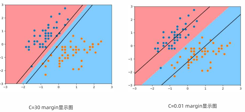
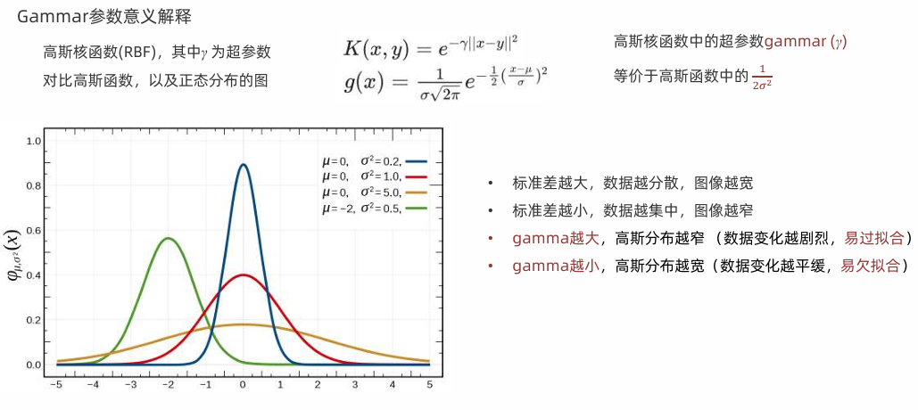
高斯核函数
高斯核 Radial Basis Function Kernel (径向基函数,又称RBF核)
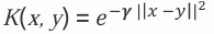
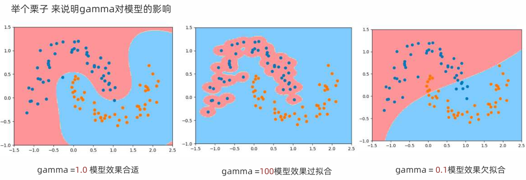
结论:gamma越大,高斯分布越窄,gamma越小,高斯分布越宽
代码实现上述案例
python
from sklearn.datasets import make_moons
import matplotlib.pyplot as plt
from sklearn.svm import SVC
from sklearn.pipeline import Pipeline
from sklearn.preprocessing import StandardScaler
from plot_util import plot_decision_boundary
import numpy as np


def dm01():
    X, y = make_moons(noise=0.15)
    print('x.shape -->', X.shape)
    print('y.shape -->', y.shape)
    plt.scatter(X[y == 0, 0], X[y == 0, 1])
    plt.scatter(X[y == 1, 0], X[y == 1, 1])
    plt.show()

    def RBFKernelSVC(gamma=1.0):
        return Pipeline([
            ('std_scaler', StandardScaler()),
            ('svc', SVC(kernel='rbf', gamma=gamma))
        ])

    print('x.shape -->', X.shape)
    print('y.shape -->', y.shape)

    svc1 = RBFKernelSVC(gamma=1.0)
    svc1.fit(X, y)

    # 画图
    plot_decision_boundary(svc1, axis=[-1.5, 2.5, -1.0, 1.5])
    plt.scatter(X[y == 0, 0], X[y == 0, 1])
    plt.scatter(X[y == 1, 0], X[y == 1, 1])
    plt.show()

    # 4.2 实例化模型2 -过拟合
    svc2 = RBFKernelSVC(gamma=100)
    svc2.fit(X, y)
    plot_decision_boundary(svc2, axis=[-1.5, 2.5, -1.0, 1.5])
    plt.scatter(X[y == 0, 0], X[y == 0, 1])
    plt.scatter(X[y == 1, 0], X[y == 1, 1])
    plt.show()

    # 4.3 实例化模型3 -欠拟合
    svc3 = RBFKernelSVC(gamma=0.1)
    svc3.fit(X, y)
    plot_decision_boundary(svc3, axis=[-1.5, 2.5, -1.0, 1.5])
    plt.scatter(X[y == 0, 0], X[y == 0, 1])
    plt.scatter(X[y == 1, 0], X[y == 1, 1])
    plt.show()


dm01()SVC和LinearSVC主要区别对比
| 特性 | SVC(kernel='linear') |
LinearSVC |
|---|---|---|
| 底层库 | libsvm | liblinear |
| 优化算法 | SMO | 坐标下降法 |
| 正则化参数 | C(惩罚系数) |
C(惩罚系数) |
| 损失函数 | 铰链损失(hinge loss) | 可选的损失函数 |
| 正则化形式 | L2 正则化 | L2 或 L1 正则化(通过 penalty) |
| 截距(bias)处理 | 自动处理 | 可选择是否拟合截距 |
| 多分类策略 | 一对一(one-vs-one) | 一对多(one-vs-rest) |
| 速度(线性问题) | 较慢 | 快很多(特别是大数据) |
| 核函数 | 支持各种核 | 仅线性 |
| 支持稀疏数据 | 有限 | 更好 |
LinearSVC基于load_iris实现多分类
python
from sklearn.datasets import load_iris
import matplotlib.pyplot as plt
from sklearn.preprocessing import StandardScaler
from sklearn.svm import LinearSVC
import numpy as np
plt.rcParams['font.sans-serif'] = ['Microsoft YaHei', 'SimHei', 'KaiTi']
plt.rcParams['axes.unicode_minus'] = False
# 如果你没有plot_decision_boundary_svc,这里是实现
def plot_decision_boundary_svc(model, axis):
"""绘制SVM决策边界"""
x0, x1 = np.meshgrid(
np.linspace(axis[0], axis[1], 500),
np.linspace(axis[2], axis[3], 500)
)
X_new = np.c_[x0.ravel(), x1.ravel()]
y_predict = model.predict(X_new)
zz = y_predict.reshape(x0.shape)
from matplotlib.colors import ListedColormap
custom_cmap = ListedColormap(['#EF9A9A', '#90CAF9', '#A5D6A7'])
plt.contourf(x0, x1, zz, cmap=custom_cmap, alpha=0.3)
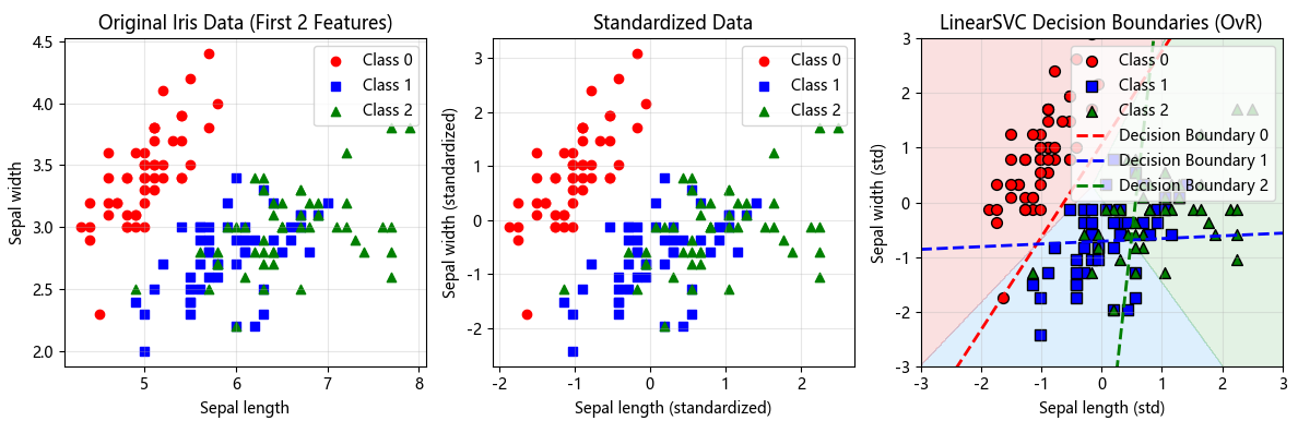
def dm01_iris_multiclass():
"""使用完整Iris数据集展示LinearSVC的多分类"""
# 1. 加载完整数据
X, y = load_iris(return_X_y=True)
print('完整数据集:')
print('X.shape -->', X.shape) # (150, 4)
print('y.shape -->', y.shape) # (150,)
print('类别分布:', np.bincount(y)) # [50, 50, 50]
print('类别标签:', np.unique(y)) # [0, 1, 2]
# 2. 可视化前两个特征(便于绘图)
plt.figure(figsize=(12, 4))
# 原始数据可视化
plt.subplot(131)
colors = ['red', 'blue', 'green']
markers = ['o', 's', '^']
for i in range(3):
plt.scatter(X[y == i, 0], X[y == i, 1],
color=colors[i], marker=markers[i],
label=f'Class {i}')
plt.xlabel('Sepal length')
plt.ylabel('Sepal width')
plt.title('Original Iris Data (First 2 Features)')
plt.legend()
plt.grid(True, alpha=0.3)
# 3. 标准化(重要!SVM对尺度敏感)
scaler = StandardScaler()
X_std = scaler.fit_transform(X)
# 标准化后可视化
plt.subplot(132)
for i in range(3):
plt.scatter(X_std[y == i, 0], X_std[y == i, 1],
color=colors[i], marker=markers[i],
label=f'Class {i}')
plt.xlabel('Sepal length (standardized)')
plt.ylabel('Sepal width (standardized)')
plt.title('Standardized Data')
plt.legend()
plt.grid(True, alpha=0.3)
# 4. 使用LinearSVC进行多分类
print('\n=== LinearSVC多分类演示 ===')
# LinearSVC默认使用One-vs-Rest策略
svc = LinearSVC(
C=1.0, # 正则化参数
dual='auto', # 自动选择对偶或原始问题
multi_class='ovr', # One-vs-Rest策略
random_state=42,
max_iter=10000
)
# 只用前两个特征训练(为了可视化)
svc.fit(X_std[:, :2], y)
print(f'训练准确率: {svc.score(X_std[:, :2], y):.4f}')
print(f'系数形状: {svc.coef_.shape}') # (3, 2) - 3个分类器,每个有2个系数
print(f'截距形状: {svc.intercept_.shape}') # (3,) - 3个截距
# 5. 可视化决策边界
plt.subplot(133)
# 绘制决策区域
plot_decision_boundary_svc(svc, axis=[-3, 3, -3, 3])
# 绘制数据点
for i in range(3):
plt.scatter(X_std[y == i, 0], X_std[y == i, 1],
color=colors[i], marker=markers[i],
edgecolor='k', s=50,
label=f'Class {i}')
# 绘制决策边界线
x_boundary = np.linspace(-3, 3, 100)
# 对于One-vs-Rest,每条线是决策函数为0的地方
# w1*x1 + w2*x2 + b = 0 => x2 = -(w1*x1 + b)/w2
for i in range(3):
w1, w2 = svc.coef_[i]
b = svc.intercept_[i]
# 注意:这里可能出现除以0的情况
if abs(w2) > 1e-10:
y_boundary = -(w1 * x_boundary + b) / w2
plt.plot(x_boundary, y_boundary,
color=colors[i], linestyle='--',
linewidth=2, label=f'Decision Boundary {i}')
plt.xlabel('Sepal length (std)')
plt.ylabel('Sepal width (std)')
plt.title('LinearSVC Decision Boundaries (OvR)')
plt.legend(loc='upper right')
plt.grid(True, alpha=0.3)
plt.axis([-3, 3, -3, 3])
plt.tight_layout()
plt.show()
# 6. 深入分析决策函数
print('\n=== 决策函数分析 ===')
# 获取三个分类器的决策值
decision_values = svc.decision_function(X_std[:5, :2]) # 前5个样本
print('前5个样本的决策值(每列对应一个分类器):')
print(decision_values)
print(f'决策值形状: {decision_values.shape}') # (5, 3)
# 预测结果
predictions = svc.predict(X_std[:5, :2])
print('预测结果:', predictions)
print('真实标签:', y[:5])
# 7. 查看One-vs-Rest如何工作
print('\n=== One-vs-Rest原理 ===')
print('分类器0: 是类别0 vs 不是类别0')
print('分类器1: 是类别1 vs 不是类别1')
print('分类器2: 是类别2 vs 不是类别2')
print('\n每个样本选择决策值最大的分类器作为最终类别')
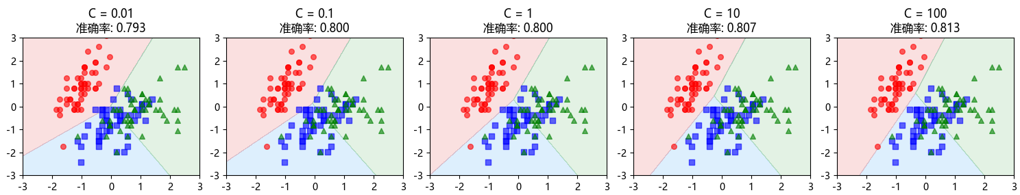
# 8. 使用不同C值对比
print('\n=== 不同C值的影响 ===')
C_values = [0.01, 0.1, 1, 10, 100]
plt.figure(figsize=(15, 3))
for idx, C in enumerate(C_values):
svc_tmp = LinearSVC(C=C, dual='auto', max_iter=10000, random_state=42)
svc_tmp.fit(X_std[:, :2], y)
plt.subplot(1, len(C_values), idx + 1)
plot_decision_boundary_svc(svc_tmp, axis=[-3, 3, -3, 3])
for i in range(3):
plt.scatter(X_std[y == i, 0], X_std[y == i, 1],
color=colors[i], marker=markers[i],
alpha=0.6, s=30)
plt.title(f'C = {C}\n准确率: {svc_tmp.score(X_std[:, :2], y):.3f}')
plt.axis([-3, 3, -3, 3])
plt.tight_layout()
plt.show()
return svc, X_std, y
# 运行函数
if __name__ == '__main__':
svc_model, X_standardized, y_labels = (dm01_iris_multiclass())