从头开始学习AI：第五章 - 多分类与正则化技术

回顾与引言

在前四章中，我们学习了线性回归和逻辑回归的基础知识。本章将深入探讨更高级的主题：

1. 实现多分类逻辑回归（Softmax回归）
2. 学习正则化技术在逻辑回归中的应用

1. Softmax回归（多分类逻辑回归）

Softmax回归是逻辑回归的多分类扩展，适用于目标变量有多个类别的情况。

数学原理

Softmax函数将线性输出转换为概率分布：

其中 k 是类别数量。

成本函数（交叉熵）

其中

梯度计算

代码实现：Softmax回归

import numpy as np
import matplotlib.pyplot as plt
from sklearn.datasets import make_classification
from sklearn.model_selection import train_test_split
from sklearn.preprocessing import StandardScaler, LabelBinarizer
from sklearn.linear_model import LogisticRegression as SklearnLogisticRegression
from sklearn.metrics import accuracy_score, confusion_matrix, classification_report

class SoftmaxRegression:
    """
    手动实现Softmax回归（多分类逻辑回归）
    """
    
    def __init__(self, learning_rate=0.01, n_iterations=1000, lambda_=0.1, reg_type='l2'):
        """
        初始化Softmax回归模型
        
        参数:
        learning_rate -- 学习率 α
        n_iterations -- 迭代次数
        lambda_ -- 正则化参数
        reg_type -- 正则化类型 ('l1', 'l2', 或 None)
        """
        self.learning_rate = learning_rate
        self.n_iterations = n_iterations
        self.lambda_ = lambda_
        self.reg_type = reg_type
        self.theta = None  # 参数矩阵 (n_features, n_classes)
        self.cost_history = []  # 成本函数历史
        self.n_classes = None  # 类别数量
    
    def _softmax(self, z):
        """
        Softmax函数: 将输出转换为概率分布
        
        参数:
        z -- 输入矩阵 (m, n_classes)
        
        返回:
        概率矩阵 (m, n_classes)
        """
        # 数值稳定性处理：减去最大值防止指数溢出
        exp_z = np.exp(z - np.max(z, axis=1, keepdims=True))
        return exp_z / np.sum(exp_z, axis=1, keepdims=True)
    
    def _add_intercept(self, X):
        """
        在特征矩阵前添加一列1，用于截距项
        
        参数:
        X -- 特征矩阵 (m, n)
        
        返回:
        添加截距项后的特征矩阵 (m, n+1)
        """
        intercept = np.ones((X.shape[0], 1))
        return np.concatenate((intercept, X), axis=1)
    
    def _compute_cost(self, X, y):
        """
        计算交叉熵成本函数（带正则化）
        
        参数:
        X -- 特征矩阵 (包含截距项)
        y -- 目标矩阵 (one-hot编码)
        
        返回:
        成本函数值
        """
        m = len(y)
        h = self._softmax(X.dot(self.theta))
        
        # 计算交叉熵损失
        cost = (-1 / m) * np.sum(y * np.log(h + 1e-15))  # 添加小值防止log(0)
        
        # 添加正则化项
        if self.reg_type == 'l2':
            # L2正则化: λ/2m * Σθ² (不包括截距项)
            reg_term = (self.lambda_ / (2 * m)) * np.sum(self.theta[1:, :] ** 2)
            cost += reg_term
        elif self.reg_type == 'l1':
            # L1正则化: λ/m * Σ|θ| (不包括截距项)
            reg_term = (self.lambda_ / m) * np.sum(np.abs(self.theta[1:, :]))
            cost += reg_term
        
        return cost
    
    def fit(self, X, y):
        """
        使用梯度下降训练Softmax回归模型
        
        参数:
        X -- 特征矩阵 (m, n)
        y -- 目标向量 (m,)
        """
        # 添加截距项
        X_b = self._add_intercept(X)
        
        # 获取类别信息并转换为one-hot编码
        self.n_classes = len(np.unique(y))
        lb = LabelBinarizer()
        y_onehot = lb.fit_transform(y)
        
        # 初始化参数矩阵 (n_features+1, n_classes)
        self.theta = np.zeros((X_b.shape[1], self.n_classes))
        
        m = len(y)
        self.cost_history = []
        
        # 梯度下降迭代
        for iteration in range(self.n_iterations):
            # 计算预测概率
            z = X_b.dot(self.theta)
            h = self._softmax(z)
            
            # 计算梯度
            gradient = (1 / m) * X_b.T.dot(h - y_onehot)
            
            # 添加正则化梯度
            if self.reg_type == 'l2':
                # L2正则化梯度: λ/m * θ (不包括截距项)
                reg_gradient = (self.lambda_ / m) * self.theta
                reg_gradient[0, :] = 0  # 不对截距项正则化
                gradient += reg_gradient
            elif self.reg_type == 'l1':
                # L1正则化梯度: λ/m * sign(θ) (不包括截距项)
                reg_gradient = (self.lambda_ / m) * np.sign(self.theta)
                reg_gradient[0, :] = 0  # 不对截距项正则化
                gradient += reg_gradient
            
            # 更新参数
            self.theta -= self.learning_rate * gradient
            
            # 记录成本值
            cost = self._compute_cost(X_b, y_onehot)
            self.cost_history.append(cost)
            
            # 每100次迭代打印进度
            if iteration % 100 == 0:
                print(f"Iteration {iteration}: Cost = {cost:.6f}")
    
    def predict_proba(self, X):
        """
        预测概率值
        
        参数:
        X -- 特征矩阵
        
        返回:
        预测概率矩阵 (m, n_classes)
        """
        X_b = self._add_intercept(X)
        return self._softmax(X_b.dot(self.theta))
    
    def predict(self, X):
        """
        预测类别
        
        参数:
        X -- 特征矩阵
        
        返回:
        预测类别
        """
        probabilities = self.predict_proba(X)
        return np.argmax(probabilities, axis=1)
    
    def plot_cost_history(self):
        """
        绘制成本函数下降曲线
        """
        plt.figure(figsize=(10, 6))
        plt.plot(self.cost_history)
        plt.xlabel('Iterations')
        plt.ylabel('Cost')
        plt.title('Cost Function History')
        plt.grid(True)
        plt.show()

# 示例使用
if __name__ == "__main__":
    # 生成多分类数据
    np.random.seed(42)
    X, y = make_classification(n_samples=1000, n_features=4, n_informative=4,
                              n_redundant=0, n_classes=3, n_clusters_per_class=1,
                              random_state=42)
    
    # 数据预处理
    scaler = StandardScaler()
    X_scaled = scaler.fit_transform(X)
    
    # 划分训练集和测试集
    X_train, X_test, y_train, y_test = train_test_split(
        X_scaled, y, test_size=0.2, random_state=42
    )
    
    print("数据形状:")
    print(f"训练集: {X_train.shape}, 测试集: {X_test.shape}")
    print(f"类别数量: {len(np.unique(y))}")
    
    # 训练Softmax回归模型
    print("\n=== 训练Softmax回归模型 ===")
    softmax_model = SoftmaxRegression(learning_rate=0.1, n_iterations=1000, lambda_=0.1, reg_type='l2')
    softmax_model.fit(X_train, y_train)
    
    # 训练scikit-learn多分类逻辑回归模型
    print("\n=== 训练scikit-learn多分类逻辑回归模型 ===")
    sklearn_model = SklearnLogisticRegression(multi_class='multinomial', solver='lbfgs')
    sklearn_model.fit(X_train, y_train)
    
    # 评估模型
    y_pred_softmax = softmax_model.predict(X_test)
    y_pred_sklearn = sklearn_model.predict(X_test)
    
    accuracy_softmax = accuracy_score(y_test, y_pred_softmax)
    accuracy_sklearn = accuracy_score(y_test, y_pred_sklearn)
    
    print(f"\n=== 模型评估 ===")
    print(f"Softmax回归准确率: {accuracy_softmax:.4f}")
    print(f"Scikit-learn准确率: {accuracy_sklearn:.4f}")
    
    # 可视化成本函数下降
    softmax_model.plot_cost_history()
    
    # 查看模型参数
    print(f"\nSoftmax模型参数形状: {softmax_model.theta.shape}")

数据形状:

训练集: (800, 4), 测试集: (200, 4)

类别数量: 3

=== 训练Softmax回归模型 ===

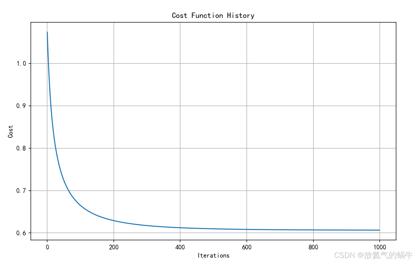
Iteration 0: Cost = 1.073610

Iteration 100: Cost = 0.664719

Iteration 200: Cost = 0.628946

Iteration 300: Cost = 0.617297

Iteration 400: Cost = 0.612204

Iteration 500: Cost = 0.609652

Iteration 600: Cost = 0.608272

Iteration 700: Cost = 0.607490

Iteration 800: Cost = 0.607035

Iteration 900: Cost = 0.606763

=== 训练scikit-learn多分类逻辑回归模型 ===

-\] /lib/python3.12/site-packages/sklearn/linear_model/_logistic.py:1247: FutureWarning: 'multi_class' was deprecated in version 1.5 and will be removed in 1.7. From then on, it will always use 'multinomial'. Leave it to its default value to avoid this warning. \[-\] warnings.warn( === 模型评估 === Softmax回归准确率: 0.7700 Scikit-learn准确率: 0.770

Softmax模型参数形状: (5, 3)

训练流程解析

一、整体结构概览

这个 SoftmaxRegression 类实现了：

• 多分类（3类及以上）
• 带 L1/L2 正则化
• 使用梯度下降优化
• 与 sklearn 的 LogisticRegression(multi_class='multinomial') 对比

它的流程依然是：

训练数据 → 损失函数 → 计算梯度 → 更新参数 θ → 收敛后得到最优 θ
                                     ↓
新样本 → 代入预测公式（Softmax）→ 输出概率 → 取最大概率类别

二、自定义类：SoftmaxRegression

1. 初始化方法：__init__

def __init__(self, learning_rate=0.01, n_iterations=1000, lambda_=0.1, reg_type='l2'):
    self.learning_rate = learning_rate
    self.n_iterations = n_iterations
    self.lambda_ = lambda_      # 正则化强度
    self.reg_type = reg_type    # 正则化类型
    self.theta = None           # 参数矩阵
    self.cost_history = []
    self.n_classes = None       # 类别数

说明：

• lambda_: 控制正则化项的权重
• reg_type: 支持 'l1' 或 'l2' 正则化，防止过拟合
• theta: 不再是向量，而是 矩阵 (n_features+1, n_classes) ------ 每一列对应一个类的参数

---

2. 私有方法：_softmax(z)

def _softmax(self, z):
    exp_z = np.exp(z - np.max(z, axis=1, keepdims=True))
    return exp_z / np.sum(exp_z, axis=1, keepdims=True)

核心公式（Softmax 函数）：

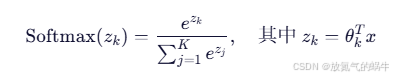
作用：

• 将线性输出 z=Xθ 转换为 概率分布
• 所有类的概率和为 1
• 数值稳定性技巧：减去每行最大值，防止 exp() 溢出

举例：若某样本的 z=[2.0,1.0,0.1]，Softmax 输出可能是 [0.65,0.25,0.10]，表示最可能是第 0 类。

---

3. 私有方法：_add_intercept(X)

def _add_intercept(self, X):
    intercept = np.ones((X.shape[0], 1))
    return np.concatenate((intercept, X), axis=1)

作用：

• 添加截距项（偏置项），即 x0=1
• 输入 (m, n) → 输出 (m, n+1)
• 使得参数矩阵 θθ 中第一行对应所有类的截距项

---

4. 私有方法：_compute_cost(X, y)

def _compute_cost(self, X, y):
    m = len(y)
    h = self._softmax(X.dot(self.theta))  # 预测概率
    cost = (-1 / m) * np.sum(y * np.log(h + 1e-15))  # 交叉熵损失

核心公式（交叉熵损失函数，多分类）：

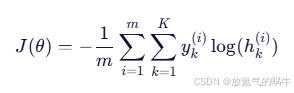
• yk(i): 第 i 个样本是否属于第 k 类（one-hot 编码）
• hk(i): 模型预测该样本属于第 k 类的概率

这就是"数据放进去训练"的那个公式！

加上正则化项：

if self.reg_type == 'l2':
    reg_term = (self.lambda_ / (2 * m)) * np.sum(self.theta[1:, :] ** 2)
    cost += reg_term
elif self.reg_type == 'l1':
    reg_term = (self.lambda_ / m) * np.sum(np.abs(self.theta[1:, :]))
    cost += reg_term

• L2 正则化：（不包括截距）
• L1 正则化：

正则化目的：防止过拟合，提升泛化能力

---

5. 训练方法：fit(X, y)

def fit(self, X, y):
    X_b = self._add_intercept(X)
    
    # 转换 y 为 one-hot 编码
    self.n_classes = len(np.unique(y))
    lb = LabelBinarizer()
    y_onehot = lb.fit_transform(y)
    
    # 初始化参数矩阵
    self.theta = np.zeros((X_b.shape[1], self.n_classes))
    
    for iteration in range(self.n_iterations):
        z = X_b.dot(self.theta)           # 线性输出 (m, K)
        h = self._softmax(z)              # 概率输出 (m, K)
        gradient = (1 / m) * X_b.T.dot(h - y_onehot)  # 基础梯度
        
        # 加上正则化梯度
        if self.reg_type == 'l2':
            reg_gradient = (self.lambda_ / m) * self.theta
            reg_gradient[0, :] = 0  # 截距项不正则化
            gradient += reg_gradient
        elif self.reg_type == 'l1':
            reg_gradient = (self.lambda_ / m) * np.sign(self.theta)
            reg_gradient[0, :] = 0
            gradient += reg_gradient
        
        # 更新参数
        self.theta -= self.learning_rate * gradient
        
        # 记录损失
        cost = self._compute_cost(X_b, y_onehot)
        self.cost_history.append(cost)

训练流程详解：

步骤	公式	说明
1️⃣ 加截距	Xb=[1,x1,x2,...,xn]	构造设计矩阵
2️⃣ One-hot 编码	y→yonehoty	把标签转为向量，如 2 → [0,0,1]
3️⃣ 初始化	θ=0	参数矩阵初始化
4️⃣ 线性输出	Z=Xbθ	每个样本对每个类有一个得分
5️⃣ Softmax	H=Softmax(Z)	得分 → 概率分布
6️⃣ 计算梯度		多分类梯度公式
7️⃣ 加正则化梯度	L2/L1 梯度	控制模型复杂度
8️⃣ 更新参数	θ:=θ−α∇J	梯度下降

训练过程：把训练数据 (X, y) 放进 交叉熵损失函数，不断调整 theta

---

6. 预测概率方法：predict_proba(X)

def predict_proba(self, X):
    X_b = self._add_intercept(X)
    return self._softmax(X_b.dot(self.theta))

• 输出：每个样本属于每个类的概率
• 使用公式：

---

7. 预测类别方法：predict(X)

def predict(self, X):
    probabilities = self.predict_proba(X)
    return np.argmax(probabilities, axis=1)

• 对每一行（一个样本）取概率最大的类别索引
• 例如 [0.1, 0.8, 0.1] → 1

---

8. 可视化方法：plot_cost_history()

• 绘制 cost_history，观察损失是否收敛

---

三、流程图

测试样本 [x1, x2, x3, x4]

↓

添加截距 → [1, x1, x2, x3, x4]

↓

计算每个类的线性得分：

score_0 = θ₀₀ + θ₁₀*x1 + ... + θ₄₀*x4

score_1 = θ₀₁ + θ₁₁*x1 + ... + θ₄₁*x4

score_2 = θ₀₂ + θ₁₂*x1 + ... + θ₄₂*x4

↓

Softmax: [e^score_0, e^score_1, e^score_2] → 归一化 → [p0, p1, p2]

↓

预测类别 = argmax([p0, p1, p2])

四、总结图解

训练阶段：

训练数据 X, y

↓

y → one-hot 编码

↓

放入 交叉熵损失函数 J(θ)

↓

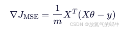
计算梯度 ∇J(θ) = (1/m) X_b^T (H - Y)

↓

更新 参数矩阵 θ

↓

直到损失最小 → 得到最优 θ

↘

→ [预测公式: P(y=k|x) = softmax(θ_k^T x)]

↗

预测阶段：

新样本 x₁,x₂,x₃,x₄\] → 代入预测公式 → 输出概率 → 取最大概率 → 输出类别

2. 正则化技术在逻辑回归中的应用

正则化是防止过拟合的重要技术，主要有两种类型：

L2正则化（岭回归）

成本函数：

梯度：

L1正则化（Lasso回归）

成本函数：

梯度（次梯度）：

代码实现：正则化

import numpy as np
import matplotlib.pyplot as plt
from sklearn.datasets import make_regression, make_classification
from sklearn.model_selection import train_test_split, learning_curve
from sklearn.preprocessing import StandardScaler, PolynomialFeatures
from sklearn.linear_model import Ridge, Lasso, ElasticNet, LogisticRegression
from sklearn.metrics import mean_squared_error, accuracy_score
from sklearn.pipeline import Pipeline

class RegularizedLinearRegression:
    """
    实现带正则化的线性回归
    """
    
    def __init__(self, regularization_type='l2', lambda_=1.0, learning_rate=0.01, n_iterations=1000):
        """
        初始化正则化线性回归模型
        
        参数:
        regularization_type -- 正则化类型: 'l1', 'l2', 'elasticnet'
        lambda_ -- 正则化强度
        learning_rate -- 学习率
        n_iterations -- 迭代次数
        """
        self.regularization_type = regularization_type
        self.lambda_ = lambda_
        self.learning_rate = learning_rate
        self.n_iterations = n_iterations
        self.theta = None
        self.cost_history = []
    
    def _add_intercept(self, X):
        """添加截距项"""
        intercept = np.ones((X.shape[0], 1))
        return np.concatenate((intercept, X), axis=1)
    
    def _compute_cost(self, X, y):
        """计算带正则化的成本函数"""
        m = len(y)
        predictions = X.dot(self.theta)
        error = predictions - y
        
        # 均方误差部分
        mse_cost = (1 / (2 * m)) * np.sum(error ** 2)
        
        # 正则化部分（不惩罚截距项）
        if self.regularization_type == 'l2':
            reg_cost = (self.lambda_ / (2 * m)) * np.sum(self.theta[1:] ** 2)
        elif self.regularization_type == 'l1':
            reg_cost = (self.lambda_ / m) * np.sum(np.abs(self.theta[1:]))
        elif self.regularization_type == 'elasticnet':
            l1_cost = (self.lambda_ / m) * np.sum(np.abs(self.theta[1:]))
            l2_cost = (self.lambda_ / (2 * m)) * np.sum(self.theta[1:] ** 2)
            reg_cost = l1_cost + l2_cost
        else:
            reg_cost = 0
        
        return mse_cost + reg_cost
    
    def _compute_gradient(self, X, y):
        """计算带正则化的梯度"""
        m = len(y)
        predictions = X.dot(self.theta)
        error = predictions - y
        
        # 基础梯度
        gradient = (1 / m) * X.T.dot(error)
        
        # 添加正则化梯度（不惩罚截距项）
        if self.regularization_type == 'l2':
            reg_gradient = (self.lambda_ / m) * self.theta
            reg_gradient[0] = 0  # 不惩罚截距项
            gradient += reg_gradient
        elif self.regularization_type == 'l1':
            reg_gradient = (self.lambda_ / m) * np.sign(self.theta)
            reg_gradient[0] = 0  # 不惩罚截距项
            gradient += reg_gradient
        elif self.regularization_type == 'elasticnet':
            l1_gradient = (self.lambda_ / m) * np.sign(self.theta)
            l2_gradient = (self.lambda_ / m) * self.theta
            reg_gradient = l1_gradient + l2_gradient
            reg_gradient[0] = 0  # 不惩罚截距项
            gradient += reg_gradient
        
        return gradient
    
    def fit(self, X, y):
        """训练模型"""
        X_b = self._add_intercept(X)
        self.theta = np.zeros(X_b.shape[1])
        self.cost_history = []
        
        for iteration in range(self.n_iterations):
            gradient = self._compute_gradient(X_b, y)
            self.theta -= self.learning_rate * gradient
            
            cost = self._compute_cost(X_b, y)
            self.cost_history.append(cost)
            
            if iteration % 100 == 0:
                print(f"Iteration {iteration}: Cost = {cost:.6f}")
    
    def predict(self, X):
        """预测"""
        X_b = self._add_intercept(X)
        return X_b.dot(self.theta)

class RegularizedLogisticRegression:
    """
    实现带正则化的逻辑回归
    """
    
    def __init__(self, regularization_type='l2', lambda_=1.0, learning_rate=0.01, n_iterations=1000):
        self.regularization_type = regularization_type
        self.lambda_ = lambda_
        self.learning_rate = learning_rate
        self.n_iterations = n_iterations
        self.theta = None
        self.cost_history = []
    
    def _sigmoid(self, z):
        return 1 / (1 + np.exp(-z))
    
    def _add_intercept(self, X):
        intercept = np.ones((X.shape[0], 1))
        return np.concatenate((intercept, X), axis=1)
    
    def _compute_cost(self, X, y):
        m = len(y)
        h = self._sigmoid(X.dot(self.theta))
        
        # 交叉熵损失
        cross_entropy = -np.mean(y * np.log(h) + (1 - y) * np.log(1 - h))
        
        # 正则化项（不惩罚截距项）
        if self.regularization_type == 'l2':
            reg_term = (self.lambda_ / (2 * m)) * np.sum(self.theta[1:] ** 2)
        elif self.regularization_type == 'l1':
            reg_term = (self.lambda_ / m) * np.sum(np.abs(self.theta[1:]))
        else:
            reg_term = 0
        
        return cross_entropy + reg_term
    
    def _compute_gradient(self, X, y):
        m = len(y)
        h = self._sigmoid(X.dot(self.theta))
        gradient = (1 / m) * X.T.dot(h - y)
        
        # 添加正则化梯度
        if self.regularization_type == 'l2':
            reg_gradient = (self.lambda_ / m) * self.theta
            reg_gradient[0] = 0
            gradient += reg_gradient
        elif self.regularization_type == 'l1':
            reg_gradient = (self.lambda_ / m) * np.sign(self.theta)
            reg_gradient[0] = 0
            gradient += reg_gradient
        
        return gradient
    
    def fit(self, X, y):
        X_b = self._add_intercept(X)
        self.theta = np.zeros(X_b.shape[1])
        self.cost_history = []
        
        for iteration in range(self.n_iterations):
            gradient = self._compute_gradient(X_b, y)
            self.theta -= self.learning_rate * gradient
            
            cost = self._compute_cost(X_b, y)
            self.cost_history.append(cost)
    
    def predict_proba(self, X):
        X_b = self._add_intercept(X)
        return self._sigmoid(X_b.dot(self.theta))
    
    def predict(self, X, threshold=0.5):
        return (self.predict_proba(X) >= threshold).astype(int)

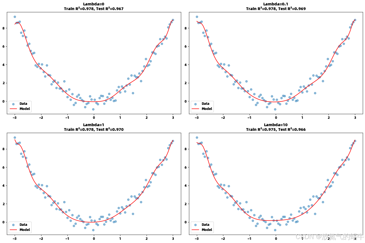
def demonstrate_overfitting():
    """演示过拟合现象"""
    np.random.seed(42)
    
    # 生成数据
    X = np.linspace(-3, 3, 100).reshape(-1, 1)
    y = X.ravel() ** 2 + np.random.normal(0, 0.5, 100)
    
    # 创建多项式特征
    poly = PolynomialFeatures(degree=15)
    X_poly = poly.fit_transform(X)
    
    # 划分训练测试集
    X_train, X_test, y_train, y_test = train_test_split(X_poly, y, test_size=0.3, random_state=42)
    
    # 训练不同正则化强度的模型
    lambdas = [0, 0.1, 1, 10]
    models = []
    
    for lambda_ in lambdas:
        model = Ridge(alpha=lambda_)
        model.fit(X_train, y_train)
        models.append(model)
        
        train_score = model.score(X_train, y_train)
        test_score = model.score(X_test, y_test)
        print(f"Lambda={lambda_}: Train R²={train_score:.3f}, Test R²={test_score:.3f}")
    
    # 绘制结果
    plt.figure(figsize=(15, 10))
    X_plot = np.linspace(-3, 3, 100).reshape(-1, 1)
    X_plot_poly = poly.transform(X_plot)
    
    for i, (lambda_, model) in enumerate(zip(lambdas, models)):
        plt.subplot(2, 2, i+1)
        plt.scatter(X, y, alpha=0.5, label='Data')
        plt.plot(X_plot, model.predict(X_plot_poly), 'r-', label='Model')
        plt.title(f'Lambda={lambda_}\nTrain R²={model.score(X_train, y_train):.3f}, Test R²={model.score(X_test, y_test):.3f}')
        plt.legend()
    
    plt.tight_layout()
    plt.show()

def compare_regularization_methods():
    """比较不同正则化方法"""
    # 生成高维数据
    X, y = make_regression(n_samples=100, n_features=100, n_informative=10, noise=0.1, random_state=42)
    X_train, X_test, y_train, y_test = train_test_split(X, y, test_size=0.3, random_state=42)
    
    # 不同正则化方法
    methods = {
        'No Regularization': RegularizedLinearRegression(regularization_type='none', lambda_=0),
        'L2 (Ridge)': RegularizedLinearRegression(regularization_type='l2', lambda_=1.0),
        'L1 (Lasso)': RegularizedLinearRegression(regularization_type='l1', lambda_=0.1),
    }
    
    results = {}
    for name, model in methods.items():
        model.fit(X_train, y_train)
        train_pred = model.predict(X_train)
        test_pred = model.predict(X_test)
        
        train_mse = mean_squared_error(y_train, train_pred)
        test_mse = mean_squared_error(y_test, test_pred)
        
        results[name] = {
            'train_mse': train_mse,
            'test_mse': test_mse,
            'theta': model.theta
        }
        
        print(f"{name}: Train MSE={train_mse:.4f}, Test MSE={test_mse:.4f}")
    
    # 绘制参数大小比较
    plt.figure(figsize=(12, 6))
    for i, (name, result) in enumerate(results.items()):
        plt.subplot(1, 3, i+1)
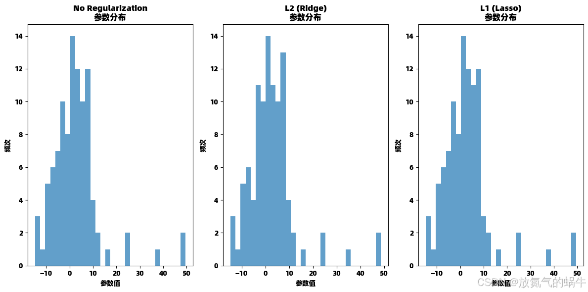
        plt.hist(result['theta'][1:], bins=30, alpha=0.7)
        plt.title(f'{name}\n参数分布')
        plt.xlabel('参数值')
        plt.ylabel('频次')
    
    plt.tight_layout()
    plt.show()
    
    return results

def plot_learning_curves():
    """绘制学习曲线"""
    X, y = make_regression(n_samples=100, n_features=1, noise=0.1, random_state=42)
    
    train_sizes = np.linspace(0.1, 1.0, 10)
    train_scores = []
    test_scores = []
    
    for train_size in train_sizes:
        size = int(train_size * len(X))
        X_train, y_train = X[:size], y[:size]
        
        model = Ridge(alpha=1.0)
        model.fit(X_train, y_train)
        
        train_scores.append(model.score(X_train, y_train))
        test_scores.append(model.score(X, y))
    
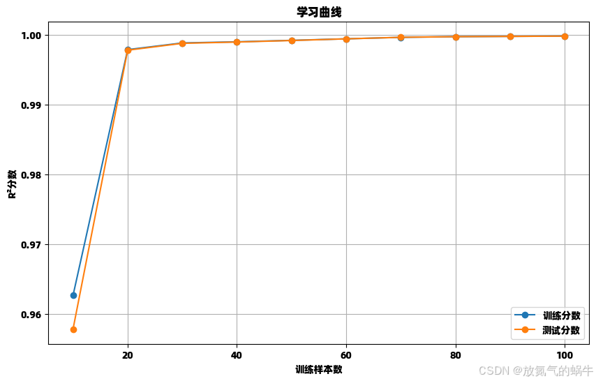
    plt.figure(figsize=(10, 6))
    plt.plot(train_sizes * len(X), train_scores, 'o-', label='训练分数')
    plt.plot(train_sizes * len(X), test_scores, 'o-', label='测试分数')
    plt.xlabel('训练样本数')
    plt.ylabel('R²分数')
    plt.title('学习曲线')
    plt.legend()
    plt.grid(True)
    plt.show()

# 示例使用
if __name__ == "__main__":
    print("=== 演示过拟合现象 ===")
    demonstrate_overfitting()
    
    print("\n=== 比较正则化方法 ===")
    results = compare_regularization_methods()
    
    print("\n=== 绘制学习曲线 ===")
    plot_learning_curves()
    
    # 逻辑回归正则化示例
    print("\n=== 逻辑回归正则化 ===")
    X, y = make_classification(n_samples=100, n_features=20, n_informative=5, random_state=42)
    X_train, X_test, y_train, y_test = train_test_split(X, y, test_size=0.3, random_state=42)
    
    # 标准化数据
    scaler = StandardScaler()
    X_train_scaled = scaler.fit_transform(X_train)
    X_test_scaled = scaler.transform(X_test)
    
    # 训练不同正则化强度的逻辑回归
    for lambda_ in [0, 0.1, 1, 10]:
        model = RegularizedLogisticRegression(regularization_type='l2', lambda_=lambda_)
        model.fit(X_train_scaled, y_train)
        
        train_acc = accuracy_score(y_train, model.predict(X_train_scaled))
        test_acc = accuracy_score(y_test, model.predict(X_test_scaled))
        
        print(f"Lambda={lambda_}: Train Acc={train_acc:.3f}, Test Acc={test_acc:.3f}")

=== 演示过拟合现象 ===

Lambda=0: Train R²=0.978, Test R²=0.967

Lambda=0.1: Train R²=0.978, Test R²=0.969

Lambda=1: Train R²=0.978, Test R²=0.970

Lambda=10: Train R²=0.975, Test R²=0.966

=== 比较正则化方法 ===

Iteration 0: Cost = 9690.857737

Iteration 100: Cost = 496.288737

Iteration 200: Cost = 187.405795

Iteration 300: Cost = 105.408628

Iteration 400: Cost = 69.986436

Iteration 500: Cost = 50.450349

Iteration 600: Cost = 37.961404

Iteration 700: Cost = 29.270814

Iteration 800: Cost = 22.923681

Iteration 900: Cost = 18.151277

No Regularization: Train MSE=29.0523, Test MSE=9051.8558

Iteration 0: Cost = 9690.897007

Iteration 100: Cost = 550.161090

Iteration 200: Cost = 253.243035

Iteration 300: Cost = 176.796888

Iteration 400: Cost = 144.740938

Iteration 500: Cost = 127.569600

Iteration 600: Cost = 116.902674

Iteration 700: Cost = 109.687672

Iteration 800: Cost = 104.564992

Iteration 900: Cost = 100.820361

L2 (Ridge): Train MSE=38.6537, Test MSE=9037.9862

Iteration 0: Cost = 9690.881719

Iteration 100: Cost = 497.123914

Iteration 200: Cost = 188.303378

Iteration 300: Cost = 106.328689

Iteration 400: Cost = 70.927166

Iteration 500: Cost = 51.406526

Iteration 600: Cost = 38.930708

Iteration 700: Cost = 30.250578

Iteration 800: Cost = 23.912109

Iteration 900: Cost = 19.146383

L1 (Lasso): Train MSE=29.0818, Test MSE=9034.9739

=== 绘制学习曲线 ===

=== 逻辑回归正则化 ===

Lambda=0: Train Acc=0.829, Test Acc=0.800

Lambda=0.1: Train Acc=0.829, Test Acc=0.800

Lambda=1: Train Acc=0.843, Test Acc=0.800

Lambda=10: Train Acc=0.814, Test Acc=0.767

训练流程解析

一、整体结构概览

模块	功能
RegularizedLinearRegression	手动实现带 L1/L2/ElasticNet 正则化的线性回归
RegularizedLogisticRegression	手动实现带 L1/L2 正则化的逻辑回归
demonstrate_overfitting()	展示高阶多项式+无正则化 → 过拟合
compare_regularization_methods()	对比不同正则化对参数的影响
plot_learning_curves()	绘制学习曲线，判断模型是否收敛
if __name__ == "__main__":	主程序，运行所有演示

---

二、第一部分：带正则化的线性回归

class RegularizedLinearRegression:
    def __init__(...): ...
    def _add_intercept(self, X): ...
    def _compute_cost(self, X, y): ...
    def _compute_gradient(self, X, y): ...
    def fit(self, X, y): ...
    def predict(self, X): ...

---

1. _add_intercept(X)

def _add_intercept(self, X):
    intercept = np.ones((X.shape[0], 1))
    return np.concatenate((intercept, X), axis=1)

作用： 添加截距项 x0=1

• 输入：(m, n) → 输出：(m, n+1)
• 使得模型可以学习偏置项 θ0θ0

---

2. _compute_cost(X, y)：损失函数（关键！）

mse_cost = (1 / (2 * m)) * np.sum(error ** 2)

核心公式（MSE 损失）：

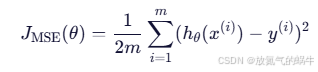
其中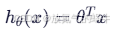

---

3. _compute_gradient(X, y)：梯度计算

gradient = (1 / m) * X.T.dot(error)  # 基础梯度

基础梯度（MSE）：