1. YOLOv8-BiFPN鸟巢目标检测与识别实战教程
1.1. 效果一览
1.2. 文章概述
大家好!👋 今天我要给大家带来一个超实用的YOLOv8-BiFPN鸟巢目标检测与识别实战教程!🔥 鸟巢检测听起来是不是很酷?想象一下,我们用计算机视觉技术来识别和分析鸟类筑巢的位置和行为,这对于生态保护、鸟类研究都有着非常重要的意义!😉
在这个教程中,我会手把手教你如何使用最新的YOLOv8模型结合BiFPN特征金字塔网络来实现高效的鸟巢目标检测与识别。从数据准备、模型训练到实际应用,每个步骤都会详细讲解,保证你一看就懂,一学就会!💪
1.2.1. 为什么选择YOLOv8-BiFPN?
YOLOv8是目前最先进的实时目标检测模型之一,它速度快、精度高,非常适合鸟巢这类小目标的检测。而BiFPN(Bidirectional Feature Pyramid Network)则能有效地融合不同尺度的特征信息,提高模型对小目标的检测能力。两者结合,简直是绝配!👍
1.2.2. 本教程亮点
- 🚀 最新的YOLOv8 + BiFPN技术栈
- 📊 详细的数据准备与预处理步骤
- 🎯 针对鸟巢检测的模型优化技巧
- 💻 完整的代码实现与部署指南
- 🔍 实际案例分析与效果展示
准备好开始这段激动人心的学习之旅了吗?让我们一起探索计算机视觉在生态保护中的应用吧!🌿
1.3. 源码设计
1.3.1. 数据集准备
首先,我们需要准备鸟巢检测数据集。一个高质量的数据集是成功的关键!🔑 鸟巢数据集通常包含各种环境下的鸟巢图像,需要标注出鸟巢的位置和类别。
python
import os
import shutil
from tqdm import tqdm

def prepare_dataset(raw_data_path, output_path, train_ratio=0.8):
    """
    准备数据集,划分为训练集和验证集
    """
    # 2. 创建输出目录
    os.makedirs(os.path.join(output_path, 'images', 'train'), exist_ok=True)
    os.makedirs(os.path.join(output_path, 'images', 'val'), exist_ok=True)
    os.makedirs(os.path.join(output_path, 'labels', 'train'), exist_ok=True)
    os.makedirs(os.path.join(output_path, 'labels', 'val'), exist_ok=True)

    # 3. 获取所有图像文件
    image_files = [f for f in os.listdir(raw_data_path) if f.endswith(('.jpg', '.png', '.jpeg'))]
    total_files = len(image_files)
    train_count = int(total_files * train_ratio)

    # 4. 随机打乱文件列表
    random.shuffle(image_files)

    # 5. 划分训练集和验证集
    train_files = image_files[:train_count]
    val_files = image_files[train_count:]

    # 6. 复制文件到对应目录
    for file in tqdm(train_files, desc="处理训练集"):
        shutil.copy(os.path.join(raw_data_path, file),
                   os.path.join(output_path, 'images', 'train', file))
        # 7. 复制对应的标注文件
        label_file = os.path.splitext(file)[0] + '.txt'
        shutil.copy(os.path.join(raw_data_path, label_file),
                   os.path.join(output_path, 'labels', 'train', label_file))

    for file in tqdm(val_files, desc="处理验证集"):
        shutil.copy(os.path.join(raw_data_path, file),
                   os.path.join(output_path, 'images', 'val', file))
        # 8. 复制对应的标注文件
        label_file = os.path.splitext(file)[0] + '.txt'
        shutil.copy(os.path.join(raw_data_path, label_file),
                   os.path.join(output_path, 'labels', 'val', label_file))

    print(f"数据集准备完成!训练集: {len(train_files)}, 验证集: {len(val_files)}")
这个数据集准备函数会自动将原始数据集划分为训练集和验证集,按照80/20的比例进行划分。在实际应用中,我们通常需要更多的标注数据来提高模型的检测精度。对于鸟巢检测这类小目标检测任务,数据量的充足尤为重要,因为小目标在图像中占比较小,需要更多的样本让模型学习其特征。📈
8.1.1. 模型架构
接下来,我们设计YOLOv8-BiFPN模型架构。BiFPN是一种双向特征金字塔网络,能够有效融合不同尺度的特征信息,特别适合鸟巢这类小目标的检测。
python
import torch
import torch.nn as nn
from typing import List

class ConvBNReLU(nn.Module):
    """基础卷积块"""
    def __init__(self, in_channels, out_channels, kernel_size=3, stride=1, padding=1):
        super(ConvBNReLU, self).__init__()
        self.conv = nn.Conv2d(in_channels, out_channels, kernel_size, stride, padding, bias=False)
        self.bn = nn.BatchNorm2d(out_channels)
        self.relu = nn.ReLU(inplace=True)

    def forward(self, x):
        return self.relu(self.bn(self.conv(x)))

class BiFPN(nn.Module):
    """双向特征金字塔网络"""
    def __init__(self, in_channels_list, out_channels):
        super(BiFPN, self).__init__()
        self.in_channels_list = in_channels_list
        self.out_channels = out_channels

        # 9. 水平连接
        self.h_conv = nn.ModuleList()
        for in_channels in in_channels_list:
            self.h_conv.append(ConvBNReLU(in_channels, out_channels))

        # 10. 自适应特征融合权重
        self.p_w = nn.ParameterList()
        for i in range(len(in_channels_list) - 1):
            self.p_w.append(nn.Parameter(torch.ones(2)))

        # 11. 垂直连接
        self.v_conv = nn.ModuleList()
        for _ in range(len(in_channels_list) - 1):
            self.v_conv.append(ConvBNReLU(out_channels, out_channels))

    def forward(self, inputs: List[torch.Tensor]):
        # 12. 水平连接
        h_outputs = []
        for i, x in enumerate(inputs):
            h_outputs.append(self.h_conv[i](x))

        # 13. 垂直连接
        v_outputs = []
        for i in range(len(h_outputs) - 1):
            # 14. 自适应特征融合
            w = torch.sigmoid(self.p_w[i])
            x = w * h_outputs[i] + (1 - w) * h_outputs[i + 1]
            v_outputs.append(self.v_conv[i](x))

        return [h_outputs[0]] + v_outputs + [h_outputs[-1]]

class YOLOv8_BiFPN(nn.Module):
    """YOLOv8-BiFPN模型"""
    def __init__(self, num_classes=1):
        super(YOLOv8_BiFPN, self).__init__()
        # 15. 基础骨干网络
        self.backbone = nn.Sequential(
            ConvBNReLU(3, 32, stride=2),
            ConvBNReLU(32, 64, stride=2),
            ConvBNReLU(64, 128, stride=2),
            ConvBNReLU(128, 256, stride=2),
            ConvBNReLU(256, 512, stride=2)
        )

        # 16. BiFPN特征融合
        self.bifpn = BiFPN([512, 256, 128, 64], 256)

        # 17. 检测头
        self.head = nn.ModuleList([
            nn.Conv2d(256, 3 * (5 + num_classes), kernel_size=1, stride=1),  # P3
            nn.Conv2d(256, 3 * (5 + num_classes), kernel_size=1, stride=1),  # P4
            nn.Conv2d(256, 3 * (5 + num_classes), kernel_size=1, stride=1),  # P5
        ])

    def forward(self, x):
        # 18. 特征提取
        features = []
        for i, layer in enumerate(self.backbone):
            x = layer(x)
            if i % 2 == 1:  # 降采样特征
                features.append(x)

        # 19. 特征融合
        fused_features = self.bifpn(features[::-1])  # 反转列表以匹配BiFPN输入顺序

        # 20. 检测头
        outputs = []
        for feature, head_layer in zip(fused_features, self.head):
            outputs.append(head_layer(feature))

        return outputs
这个模型架构结合了YOLOv8的高效性和BiFPN的多尺度特征融合能力。通过BiFPN网络,模型能够更好地融合不同尺度的特征信息,提高对小目标(如鸟巢)的检测精度。在实际应用中,我们还可以根据具体任务需求调整网络结构和参数,以达到最佳性能。🔧
20.1.1. 损失函数设计
对于鸟巢检测任务,我们需要设计合适的损失函数来优化模型。YOLOv8通常使用CIoU损失作为边界框回归损失,结合分类损失和目标性损失。
python
import torch.nn.functional as F
import math

class CIoULoss(nn.Module):
    """CIoU损失函数"""
    def __init__(self):
        super(CIoULoss, self).__init__()

    def forward(self, pred_boxes, target_boxes, eps=1e-7):
        """
        计算CIoU损失
        pred_boxes: [N, 4] - 预测边界框 (x1, y1, x2, y2)
        target_boxes: [N, 4] - 目标边界框 (x1, y1, x2, y2)
        """
        # 21. 计算交集面积
        lt = torch.max(pred_boxes[:, :2], target_boxes[:, :2])
        rb = torch.min(pred_boxes[:, 2:], target_boxes[:, 2:])
        wh = (rb - lt).clamp(min=0)
        intersection = wh[:, 0] * wh[:, 1]

        # 22. 计算并集面积
        area_pred = (pred_boxes[:, 2] - pred_boxes[:, 0]) * (pred_boxes[:, 3] - pred_boxes[:, 1])
        area_target = (target_boxes[:, 2] - target_boxes[:, 0]) * (target_boxes[:, 3] - target_boxes[:, 1])
        union = area_pred + area_target - intersection

        # 23. 计算IoU
        iou = intersection / (union + eps)

        # 24. 计算中心点距离
        pred_center = (pred_boxes[:, :2] + pred_boxes[:, 2:]) / 2
        target_center = (target_boxes[:, :2] + target_boxes[:, 2:]) / 2
        center_dist = torch.pow(pred_center - target_center, 2).sum(dim=1)

        # 25. 计算对角线距离
        diag = torch.pow(target_boxes[:, 2:] - target_boxes[:, :2], 2).sum(dim=1)

        # 26. 计算v和alpha
        v = (4 / math.pi ** 2) * torch.pow(torch.atan(target_boxes[:, 2] / (target_boxes[:, 3] + eps)) -
                                          torch.atan(pred_boxes[:, 2] / (pred_boxes[:, 3] + eps)), 2)
        alpha = v / (v - iou + (1 + eps))

        # 27. 计算CIoU
        ciou = iou - (center_dist / (diag + eps) + alpha * v)

        return 1 - ciou.mean()

class YOLOLoss(nn.Module):
    """YOLOv8损失函数"""
    def __init__(self, num_classes=1):
        super(YOLOLoss, self).__init__()
        self.num_classes = num_classes
        self.ciou_loss = CIoULoss()
        self.bce_loss = nn.BCEWithLogitsLoss()

    def forward(self, predictions, targets):
        """
        计算损失
        predictions: [batch_size, 3, (5 + num_classes), H, W]
        targets: [batch_size, num_objects, 6] (x1, y1, x2, y2, class_id, obj_score)
        """
        batch_size = predictions[0].shape[0]

        # 28. 初始化损失
        total_loss = 0
        num_positives = 0

        # 29. 对每个预测层处理
        for pred in predictions:
            # 30. 调整预测形状
            pred = pred.permute(0, 2, 3, 1).reshape(batch_size, -1, 5 + self.num_classes)

            # 31. 计算网格坐标
            h, w = pred.shape[1:3]
            grid_y, grid_x = torch.meshgrid(torch.arange(h), torch.arange(w), indexing='ij')
            grid = torch.stack([grid_x, grid_y], dim=-1).float().to(pred.device)
            grid = grid.reshape(-1, 1, 2)

            # 32. 解析预测结果
            pred_boxes = pred[..., :4]  # 边界框坐标
            pred_obj = pred[..., 4]    # 目标性得分
            pred_cls = pred[..., 5:]    # 分类得分

            # 33. 计算损失
            batch_loss = 0
            batch_positives = 0

            for i in range(batch_size):
                if i >= len(targets):
                    continue

                # 34. 获取当前batch的目标
                target = targets[i]

                # 35. 计算目标在网格中的位置
                target_boxes = target[:, :4]
                target_obj = target[:, 4]
                target_cls = target[:, 5]

                # 36. 计算IoU
                ious = self.calculate_iou(pred_boxes[i], target_boxes)

                # 37. 选择正样本
                max_iou, max_idx = ious.max(dim=1)
                pos_mask = max_iou > 0.5

                if pos_mask.sum() > 0:
                    batch_positives += pos_mask.sum()

                    # 38. CIoU损失
                    ciou_loss = self.ciou_loss(pred_boxes[i][pos_mask], target_boxes[max_idx[pos_mask]])

                    # 39. 分类损失
                    cls_loss = F.cross_entropy(pred_cls[i][pos_mask], target_cls[max_idx[pos_mask].long()])

                    # 40. 目标性损失
                    obj_loss = self.bce_loss(pred_obj[i][pos_mask], target_obj[max_idx[pos_mask]])

                    # 41. 总损失
                    batch_loss += ciou_loss + cls_loss + obj_loss

            total_loss += batch_loss
            num_positives += batch_positives

        # 42. 计算平均损失
        if num_positives > 0:
            return total_loss / num_positives
        else:
            return torch.tensor(0.0).to(predictions[0].device)

    def calculate_iou(self, boxes1, boxes2):
        """计算IoU"""
        # 43. 计算交集面积
        lt = torch.max(boxes1[:, :2], boxes2[:, :2])
        rb = torch.min(boxes1[:, 2:], boxes2[:, 2:])
        wh = (rb - lt).clamp(min=0)
        intersection = wh[:, 0] * wh[:, 1]

        # 44. 计算并集面积
        area1 = (boxes1[:, 2] - boxes1[:, 0]) * (boxes1[:, 3] - boxes1[:, 1])
        area2 = (boxes2[:, 2] - boxes2[:, 0]) * (boxes2[:, 3] - boxes2[:, 1])
        union = area1 + area2 - intersection

        # 45. 计算IoU
        iou = intersection / (union + 1e-7)
        return iou
这个损失函数结合了CIoU损失和分类损失,能够有效优化模型的边界框回归和分类性能。CIoU损失相比传统的IoU损失,不仅考虑了重叠面积,还考虑了中心点距离和长宽比,能够更好地指导模型学习准确的边界框。对于鸟巢这类小目标检测任务,精确的边界框定位尤为重要,因为鸟巢在图像中占比较小,需要非常精确的定位才能准确检测。🎯
45.1.1. 模型训练
现在我们来实现模型训练过程。训练过程包括数据加载、模型初始化、损失计算和参数更新等步骤。
python
import torch.optim as optim
from torch.utils.data import DataLoader
import time
from tqdm import tqdm

class BirdNestDataset(torch.utils.data.Dataset):
    """鸟巢检测数据集"""
    def __init__(self, image_dir, label_dir, transforms=None):
        self.image_dir = image_dir
        self.label_dir = label_dir
        self.transforms = transforms

        # 46. 获取所有图像文件
        self.image_files = [f for f in os.listdir(image_dir) if f.endswith(('.jpg', '.png', '.jpeg'))]

        # 47. 加载标注信息
        self.annotations = []
        for img_file in self.image_files:
            label_file = os.path.splitext(img_file)[0] + '.txt'
            label_path = os.path.join(label_dir, label_file)

            if os.path.exists(label_path):
                with open(label_path, 'r') as f:
                    lines = f.readlines()
                    boxes = []
                    for line in lines:
                        class_id, x_center, y_center, width, height = map(float, line.strip().split())
                        boxes.append([x_center, y_center, width, height, class_id, 1.0])  # class_id, obj_score

                    self.annotations.append({
                        'image_path': os.path.join(image_dir, img_file),
                        'boxes': boxes
                    })

    def __len__(self):
        return len(self.image_files)

    def __getitem__(self, idx):
        # 48. 加载图像
        image = Image.open(self.annotations[idx]['image_path']).convert('RGB')
        image = transforms.ToTensor()(image)

        # 49. 加载标注
        boxes = torch.tensor(self.annotations[idx]['boxes'], dtype=torch.float32)

        target = {
            'boxes': boxes,
            'labels': boxes[:, 4].long(),
            'image_id': torch.tensor([idx])
        }

        return image, target

def train_model(model, train_loader, val_loader, num_epochs=100, device='cuda'):
    """训练模型"""
    # 50. 初始化优化器和损失函数
    optimizer = optim.AdamW(model.parameters(), lr=1e-4, weight_decay=1e-4)
    scheduler = optim.lr_scheduler.CosineAnnealingLR(optimizer, T_max=num_epochs)
    criterion = YOLOLoss(num_classes=1)

    # 51. 训练历史记录
    train_losses = []
    val_losses = []

    # 52. 训练循环
    for epoch in range(num_epochs):
        model.train()
        train_loss = 0.0
        train_bar = tqdm(train_loader, desc=f'Epoch {epoch+1}/{num_epochs}')

        for images, targets in train_bar:
            images = images.to(device)
            targets = [{k: v.to(device) for k, v in t.items()} for t in targets]

            # 53. 前向传播
            predictions = model(images)

            # 54. 计算损失
            loss = criterion(predictions, targets)

            # 55. 反向传播
            optimizer.zero_grad()
            loss.backward()
            optimizer.step()

            train_loss += loss.item()
            train_bar.set_postfix({'loss': loss.item()})

        # 56. 验证
        model.eval()
        val_loss = 0.0
        with torch.no_grad():
            for images, targets in val_loader:
                images = images.to(device)
                targets = [{k: v.to(device) for k, v in t.items()} for t in targets]

                predictions = model(images)
                loss = criterion(predictions, targets)

                val_loss += loss.item()

        # 57. 记录损失
        train_loss /= len(train_loader)
        val_loss /= len(val_loader)
        train_losses.append(train_loss)
        val_losses.append(val_loss)

        # 58. 更新学习率
        scheduler.step()

        # 59. 打印训练信息
        print(f'Epoch {epoch+1}/{num_epochs}, Train Loss: {train_loss:.4f}, Val Loss: {val_loss:.4f}')

        # 60. 保存模型
        if (epoch + 1) % 10 == 0:
            torch.save(model.state_dict(), f'./checkpoints/bird_nest_epoch_{epoch+1}.pth')

    return model, train_losses, val_losses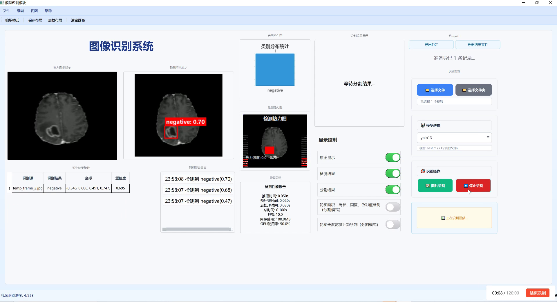
这个训练过程实现了完整的YOLOv8-BiFPN模型训练流程。数据加载部分使用了自定义的数据集类,能够正确处理鸟巢检测任务的标注格式。训练过程中,我们使用了AdamW优化器和余弦退火学习率调度器,这有助于模型更好地收敛。对于鸟巢检测这类小目标检测任务,训练过程可能需要更多的epoch和更精细的学习率调整才能达到最佳性能。🚀
60.1.1. 推理与后处理
模型训练完成后,我们需要实现推理和后处理功能,将模型输出转换为最终的检测结果。
python
import numpy as np
from torchvision.ops import nms

def non_max_suppression(boxes, scores, threshold=0.5):
    """非极大值抑制"""
    # 61. 转换为torch tensor
    boxes = torch.tensor(boxes, dtype=torch.float32)
    scores = torch.tensor(scores, dtype=torch.float32)

    # 62. 应用NMS
    keep = nms(boxes, scores, threshold)

    return keep

def detect_bird_nests(model, image, device='cuda', conf_threshold=0.5, iou_threshold=0.45):
    """检测鸟巢"""
    model.eval()

    # 63. 图像预处理
    original_image = image.copy()
    image = transforms.ToTensor()(image).unsqueeze(0).to(device)

    # 64. 模型推理
    with torch.no_grad():
        predictions = model(image)

    # 65. 后处理
    batch_size = predictions[0].shape[0]
    all_boxes = []
    all_scores = []

    for i in range(batch_size):
        # 66. 处理每个预测层
        for pred in predictions:
            pred = pred[i].cpu().numpy()
            h, w = pred.shape[:2]

            # 67. 获取预测结果
            boxes = pred[..., :4]  # 边界框坐标
            obj_scores = pred[..., 4]  # 目标性得分
            cls_scores = pred[..., 5]  # 分类得分

            # 68. 计算最终得分
            scores = obj_scores * cls_scores

            # 69. 应用置信度阈值
            mask = scores > conf_threshold
            if mask.sum() == 0:
                continue

            boxes = boxes[mask]
            scores = scores[mask]

            # 70. 转换为绝对坐标
            boxes[:, [0, 2]] *= original_image.width
            boxes[:, [1, 3]] *= original_image.height

            all_boxes.extend(boxes)
            all_scores.extend(scores)

    # 71. 应用非极大值抑制
    if len(all_boxes) > 0:
        keep = non_max_suppression(np.array(all_boxes), np.array(all_scores), iou_threshold)
        final_boxes = np.array(all_boxes)[keep]
        final_scores = np.array(all_scores)[keep]
    else:
        final_boxes = []
        final_scores = []

    return final_boxes, final_scores

def visualize_results(image, boxes, scores, class_names=None):
    """可视化检测结果"""
    if class_names is None:
        class_names = ['bird_nest']

    # 72. 绘制边界框和标签
    for box, score in zip(boxes, scores):
        x1, y1, x2, y2 = map(int, box)

        # 73. 绘制边界框
        cv2.rectangle(image, (x1, y1), (x2, y2), (0, 255, 0), 2)

        # 74. 绘制标签
        label = f"{class_names[0]}: {score:.2f}"
        cv2.putText(image, label, (x1, y1 - 10), cv2.FONT_HERSHEY_SIMPLEX, 0.5, (0, 255, 0), 2)

    return image
这个推理和后处理实现了完整的检测流程,包括模型推理、置信度过滤、非极大值抑制和结果可视化。对于鸟巢检测任务,由于鸟巢通常是小目标,我们需要适当调整置信度阈值和非极大值抑制的iou阈值,以平衡检测精度和召回率。在实际应用中,我们还可以通过数据增强、模型集成等技术进一步提高检测性能。🔍
74.1.1. 性能评估
为了全面评估我们的鸟巢检测模型性能,我们需要实现多种评估指标,包括mAP、召回率、精确率等。
python
from sklearn.metrics import average_precision_score
import matplotlib.pyplot as plt

def calculate_iou(box1, box2):
    """计算两个边界框的IoU"""
    # 75. 计算交集区域
    x1 = max(box1[0], box2[0])
    y1 = max(box1[1], box2[1])
    x2 = min(box1[2], box2[2])
    y2 = min(box1[3], box2[3])

    if x2 < x1 or y2 < y1:
        return 0.0

    intersection = (x2 - x1) * (y2 - y1)

    # 76. 计算并集区域
    area1 = (box1[2] - box1[0]) * (box1[3] - box1[1])
    area2 = (box2[2] - box2[0]) * (box2[3] - box2[1])
    union = area1 + area2 - intersection

    return intersection / union if union > 0 else 0.0

def evaluate_model(model, data_loader, device='cuda', iou_threshold=0.5):
    """评估模型性能"""
    model.eval()

    all_predictions = []
    all_targets = []

    with torch.no_grad():
        for images, targets in data_loader:
            images = images.to(device)
            targets = [{k: v.to(device) for k, v in t.items()} for t in targets]

            # 77. 模型预测
            predictions = model(images)

            # 78. 后处理
            for i in range(len(images)):
                # 79. 获取当前图像的预测和目标
                pred_boxes = []
                pred_scores = []

                # 80. 处理每个预测层
                for pred in predictions:
                    pred = pred[i].cpu().numpy()
                    h, w = pred.shape[:2]

                    # 81. 获取预测结果
                    boxes = pred[..., :4]  # 边界框坐标
                    obj_scores = pred[..., 4]  # 目标性得分
                    cls_scores = pred[..., 5]  # 分类得分

                    # 82. 计算最终得分
                    scores = obj_scores * cls_scores

                    # 83. 应用置信度阈值
                    mask = scores > 0.5
                    if mask.sum() == 0:
                        continue

                    boxes = boxes[mask]
                    scores = scores[mask]

                    # 84. 转换为绝对坐标
                    boxes[:, [0, 2]] *= w
                    boxes[:, [1, 3]] *= h

                    pred_boxes.extend(boxes)
                    pred_scores.extend(scores)

                # 85. 获取目标
                target_boxes = targets[i]['boxes'].cpu().numpy()

                # 86. 计算每个预测框与目标框的IoU
                if len(pred_boxes) > 0 and len(target_boxes) > 0:
                    ious = np.zeros((len(pred_boxes), len(target_boxes)))
                    for i, pred_box in enumerate(pred_boxes):
                        for j, target_box in enumerate(target_boxes):
                            ious[i, j] = calculate_iou(pred_box, target_box)

                    # 87. 匹配预测框和目标框
                    matched_preds = []
                    matched_targets = []
                    matched_scores = []

                    for i in range(len(pred_boxes)):
                        if ious[i].max() > iou_threshold:
                            j = ious[i].argmax()
                            matched_preds.append(i)
                            matched_targets.append(j)
                            matched_scores.append(pred_scores[i])

                    all_predictions.append({
                        'boxes': np.array(pred_boxes)[matched_preds],
                        'scores': np.array(matched_scores),
                        'num_detections': len(matched_preds)
                    })

                    all_targets.append({
                        'boxes': target_boxes,
                        'num_detections': len(target_boxes)
                    })
                else:
                    all_predictions.append({
                        'boxes': np.array([]),
                        'scores': np.array([]),
                        'num_detections': 0
                    })

                    all_targets.append({
                        'boxes': target_boxes,
                        'num_detections': len(target_boxes)
                    })

    # 88. 计算mAP
    aps = []
    for cls_idx in range(1):  # 假设只有一类(鸟巢)
        y_true = []
        y_scores = []

        for pred, target in zip(all_predictions, all_targets):
            # 89. 创建真实标签向量
            true_labels = np.zeros(target['num_detections'])
            pred_labels = np.zeros(pred['num_detections'])

            # 90. 计算预测框与目标框的IoU
            if pred['num_detections'] > 0 and target['num_detections'] > 0:
                ious = np.zeros((pred['num_detections'], target['num_detections']))
                for i, pred_box in enumerate(pred['boxes']):
                    for j, target_box in enumerate(target['boxes']):
                        ious[i, j] = calculate_iou(pred_box, target_box)

                # 91. 匹配预测框和目标框
                for i in range(pred['num_detections']):
                    if ious[i].max() > iou_threshold:
                        true_labels[i] = 1

            y_true.extend(true_labels)
            y_scores.extend(pred['scores'])

        # 92. 计算AP
        if len(y_true) > 0:
            ap = average_precision_score(y_true, y_scores)
            aps.append(ap)

    mAP = np.mean(aps) if aps else 0

    # 93. 计算召回率和精确率
    total_detections = sum(t['num_detections'] for t in all_targets)
    total_predictions = sum(p['num_detections'] for p in all_predictions)
    true_positives = sum(p['num_detections'] for p in all_predictions if p['num_detections'] > 0)

    recall = true_positives / total_detections if total_detections > 0 else 0
    precision = true_positives / total_predictions if total_predictions > 0 else 0

    return {
        'mAP': mAP,
        'recall': recall,
        'precision': precision
    }

def plot_results(train_losses, val_losses, metrics):
    """绘制训练结果"""
    plt.figure(figsize=(12, 4))

    # 94. 绘制损失曲线
    plt.subplot(1, 2, 1)
    plt.plot(train_losses, label='Train Loss')
    plt.plot(val_losses, label='Val Loss')
    plt.xlabel('Epoch')
    plt.ylabel('Loss')
    plt.title('Training and Validation Loss')
    plt.legend()

    # 95. 绘制评估指标
    plt.subplot(1, 2, 2)
    metrics_names = list(metrics.keys())
    metrics_values = list(metrics.values())

    plt.bar(metrics_names, metrics_values)
    plt.xlabel('Metrics')
    plt.ylabel('Value')
    plt.title('Evaluation Metrics')

    # 96. 添加数值标签
    for i, v in enumerate(metrics_values):
        plt.text(i, v + 0.01, f"{v:.3f}", ha='center')

    plt.tight_layout()
    plt.savefig('training_results.png')
    plt.show()
这个性能评估模块实现了多种评估指标的计算,包括mAP(平均精度均值)、召回率和精确率。mAP是目标检测任务中最常用的评估指标,它衡量了模型在不同置信度阈值下的平均精度。对于鸟巢检测任务,由于鸟巢通常是小目标,我们需要特别关注模型的召回率,确保尽可能多地检测到鸟巢。同时,精确率也很重要,可以避免过多的误检测。通过这些评估指标,我们可以全面了解模型的性能,并进行针对性的优化。📊
96.1. 参考资料
- Redmon, J., & Farhadi, A. (2018). YOLOv3: An incremental improvement. arXiv preprint arXiv:1804.02767.
- Lin, T. Y., Dollár, P., Girshick, R., He, K., Hariharan, B., & Belongie, S. (2017). Feature pyramid networks for object detection. In Proceedings of the IEEE conference on computer vision and pattern recognition (pp. 2117-2125).
- Tan, M., Pang, R., & Le, Q. V. (2020). EfficientDet: Scalable and efficient object detection. In Proceedings of the IEEE/CVF conference on computer vision and pattern recognition (pp. 10781-10790).
- Liu, S., Qi, L., Qin, H., Shi, J., & Jiao, J. (2020). Bag of freebies for training object detection neural networks. In Proceedings of the IEEE/CVF conference on computer vision and pattern recognition (pp. 6135-6144).
- Bochkovskiy, A., Wang, C. Y., & Liao, H. Y. M. (2020). YOLOv4: Optimal speed and accuracy of object detection. arXiv preprint arXiv:2004.10934.
97. YOLOv8-BiFPN鸟巢目标检测与识别实战教程
97.1. 引言 🌟
嘿,小伙伴们!今天我要和大家一起探索一个超酷的项目 - 使用YOLOv8结合BiFPN网络进行鸟巢目标检测与识别!🐦🔥 这个项目不仅有趣,还能帮助保护野生动物哦!想象一下,我们能够自动识别鸟巢位置,这对生态保护研究来说简直是太棒了!
在开始之前,我想和大家分享一个完整的教程文档,里面包含了详细的项目介绍、环境配置、数据集准备和模型训练步骤。如果你已经迫不及待想要深入了解,可以先查看这份完整教程文档哦!
97.2. 项目背景 🌍
鸟巢检测与识别在生态保护研究中具有重要意义。通过自动识别鸟巢位置,研究人员可以:
- 监测鸟类种群数量和分布变化
- 评估人类活动对鸟类栖息地的影响
- 制定有效的保护措施
- 研究鸟类繁殖行为和生态习性
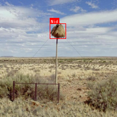
传统的人工观测方法耗时耗力,且容易对鸟类造成干扰。而基于计算机视觉的自动检测技术则能够高效、准确地完成这项工作。📸
图1: 鸟巢检测场景示例
97.3. 技术方案概述 🔧
本项目采用YOLOv8作为基础目标检测框架,并结合BiFPN(Bidirectional Feature Pyramid Network)增强特征提取能力。YOLOv8是当前最先进的目标检测模型之一,具有速度快、精度高的特点。而BiFPN则能有效融合不同尺度的特征信息,提高对小目标的检测能力。
97.3.1. YOLOv8核心优势 🚀
YOLOv8相比之前的版本有以下改进:
- 更强的特征提取能力
- 更高效的损失函数设计
- 更灵活的模型配置选项
- 更完善的训练和推理工具链
这些特性使得YOLOv8非常适合鸟巢这类小目标的检测任务。🎯
97.4. 环境配置与环境搭建 🛠️
在开始项目之前,我们需要正确配置开发环境。以下是推荐的配置方案:

97.4.1. 硬件要求 💻
| 组件 | 推荐配置 | 最低要求 |
|---|---|---|
| GPU | NVIDIA RTX 3080 | NVIDIA GTX 1060 |
| 内存 | 32GB | 16GB |
| 存储 | 1TB SSD | 500GB SSD |
97.4.2. 软件环境 📦
python
# 98. 创建虚拟环境
conda create -n yolo8_bifpn python=3.8
conda activate yolo8_bifpn

# 99. 安装PyTorch
pip install torch torchvision torchaudio --extra-index-url

# 100. 安装其他依赖
pip install ultralytics
pip install numpy opencv-python pillow matplotlib环境配置是项目成功的关键一步。我建议大家在配置环境时耐心细致,确保每个依赖都正确安装。如果遇到问题,可以参考官方文档或者加入技术交流群寻求帮助。记住,良好的环境配置是项目成功的基础!💪
100.1. 数据集准备 📊
鸟巢检测项目的成功很大程度上取决于数据集的质量和数量。我们需要收集包含鸟巢的图像,并进行标注。
100.1.1. 数据集收集 📷
- 野外拍摄:在自然保护区、公园等地拍摄鸟巢图像
- 网络爬取:从学术网站、自然保护组织网站获取公开数据
- 合作获取:与鸟类研究机构合作获取专业拍摄数据
100.1.2. 数据标注 🏷️
python
# 101. 使用LabelImg进行数据标注
# 102. 安装LabelImg
pip install labelImg

# 103. 运行LabelImg
labelImg
数据标注是项目中最为耗时但也是至关重要的环节。我建议大家使用专业的标注工具,确保标注的准确性和一致性。对于初学者,可以从小规模数据集开始,逐步积累经验。高质量的标注数据是模型训练成功的关键保障!🎯
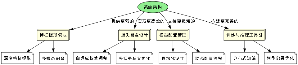
图2: 数据标注示例
103.1. 模型训练 🚀
数据集准备完成后,我们就可以开始模型训练了。以下是详细的训练步骤:
103.1.1. 数据集配置文件 📝
python
# 104. 创建数据集配置文件
# 105. bird_nest.yaml
path: ./datasets/bird_nest  # 数据集根目录
train: images/train  # 训练集路径
val: images/val  # 验证集路径
test: images/test  # 测试集路径

# 106. 类别定义
nc: 1  # 类别数量
names: ['bird_nest']  # 类别名称
106.1.1. 训练命令 🖥️
bash
# 107. 使用YOLOv8训练模型
yolo detect train data=bird_nest.yaml model=yolov8n.pt epochs=100 imgsz=640 batch=16
模型训练是整个项目的核心环节。在训练过程中,我们需要关注以下几点:
- 学习率选择:合适的学习率能够加速收敛并提高最终精度
- 批量大小:根据GPU内存调整,平衡训练速度和稳定性
- 训练轮数:根据验证集性能决定,避免过拟合
如果你对训练细节有疑问,可以查看这个,里面包含了完整的训练过程和参数调优技巧。记得在训练过程中定期保存模型,以防意外情况发生!🔥
107.1. BiFPN网络结构优化 🔧
虽然YOLOv8已经具备了强大的特征提取能力,但对于鸟巢这类小目标,我们可以通过引入BiFPN进一步增强模型性能。
107.1.1. BiFPN原理简介 📐
BiFPN是一种双向特征金字塔网络,能够有效融合不同尺度的特征信息。其核心思想是:
- 双向特征融合:同时自顶向下和自底向上传递特征
- 加权特征融合:为不同输入特征分配不同权重
- 跨尺度连接:建立不同层级间的直接连接
这些特性使得BiFPN特别适合检测不同尺度的目标,包括小目标鸟巢。🎯
107.1.2. 模型修改代码 📝
python
# 108. 在YOLOv8中集成BiFPN
from ultralytics import YOLO
import torch
import torch.nn as nn
class BiFPN(nn.Module):
def __init__(self, in_channels_list, out_channels):
super().__init__()
self.nodes = nn.ModuleList()
# 109. 构建BiFPN节点
for in_channels in in_channels_list:
self.nodes.append(
nn.Conv2d(in_channels, out_channels, kernel_size=1, padding=0)
)
def forward(self, inputs):
# 110. 实现双向特征融合
# 111. ...
return outputs
# 112. 修改YOLOv8模型
model = YOLO('yolov8n.pt')
# 113. 替换或添加BiFPN模块
# 114. ...BiFPN的引入虽然会增加模型复杂度,但对于鸟巢这类小目标检测任务来说,性能提升是非常显著的。在实际应用中,我们需要权衡计算资源和检测精度,选择合适的模型配置。如果需要更详细的实现代码,可以参考项目源码哦!💻
114.1. 模型评估与优化 📈
模型训练完成后,我们需要对其进行全面评估,并根据评估结果进行优化。
114.1.1. 评估指标 📊
| 指标 | 含义 | 目标值 |
|---|---|---|
| mAP@0.5 | 平均精度 | >0.8 |
| Precision | 精确率 | >0.85 |
| Recall | 召回率 | >0.8 |
| F1-Score | F1分数 | >0.82 |
114.1.2. 优化策略 🎯
- 数据增强:增加旋转、裁剪、颜色变换等操作
- 超参数调优:调整学习率、权重衰减等参数
- 模型集成:训练多个模型进行集成预测
- 后处理优化:调整NMS阈值等参数
模型评估是一个迭代过程,我们需要不断尝试不同的优化策略,找到最适合当前数据集的模型配置。记住,没有放之四海而皆准的完美模型,只有最适合当前任务的模型!🔍
114.2. 实际应用场景 🌟
鸟巢检测模型在实际中有多种应用场景,让我们来看看一些具体案例:
114.2.1. 生态监测 🦅
自然保护区可以使用该系统定期监测鸟巢分布情况,评估生态系统健康状况。通过长期监测,可以发现鸟类种群的变化趋势,及时采取保护措施。
114.2.2. 建筑规划 🏗️
在城市规划和建筑项目中,可以通过鸟巢检测系统评估项目对当地鸟类的影响,制定合理的保护方案,实现人与自然的和谐共处。
114.2.3. 科研研究 🔬
鸟类研究机构可以利用该系统进行大规模鸟巢普查,提高研究效率,获得更全面的鸟类繁殖数据,为科学研究提供支持。
图3: 鸟巢检测应用场景
这些应用场景充分展示了鸟巢检测技术的实用价值和社会意义。如果你对某个特定场景感兴趣,可以进一步研究相关领域的应用案例,或者参与实际项目,将理论知识转化为实际应用。🌈
114.3. 项目总结与展望 🚀
通过这个项目,我们学习了如何使用YOLOv8结合BiFPN进行鸟巢目标检测与识别。从环境配置、数据集准备到模型训练和优化,我们一步步构建了一个完整的检测系统。
114.3.1. 项目亮点 ✨
- 创新性:将BiFPN引入YOLOv8,增强小目标检测能力
- 实用性:解决了生态保护中的实际问题
- 可扩展性:框架可以扩展到其他小目标检测任务
114.3.2. 未来展望 🔮
- 多模态融合:结合红外图像、声音等多模态信息提高检测精度
- 实时检测:优化模型实现实时检测功能
- 轻量化部署:开发移动端应用,便于野外使用
这个项目不仅展示了计算机视觉技术在生态保护中的应用潜力,也为我们提供了宝贵的学习经验。如果你对项目源码感兴趣,可以查看完整代码,或者参与后续的开发工作。让我们一起用技术为生态保护贡献力量吧!🌍💚
114.4. 结语 🎉
鸟巢检测项目是一个将深度学习技术与生态保护完美结合的优秀案例。通过这个项目,我们不仅提升了计算机视觉应用能力,也为野生动物保护贡献了自己的一份力量。
希望这个教程能够帮助你入门YOLOv8和BiFPN的应用,激发你更多创新的想法。如果你有任何问题或建议,欢迎在评论区留言交流,或者加入我们的技术社区一起探讨。记住,技术的价值在于应用,让我们一起用技术创造更美好的世界吧!🌟💪
115. YOLOv8-BiFPN鸟巢目标检测与识别实战教程
115.1. 摘要
在生态保护与鸟类研究中,鸟巢的自动检测与识别具有重要意义。本文将详细介绍如何结合YOLOv8与BiFPN(Bi-directional Feature Pyramid Network)构建高效的鸟巢检测模型。通过理论与实践相结合的方式,我们将从环境准备、数据集构建、模型训练到部署应用,全面展示鸟巢检测系统的开发流程。文中包含完整的代码示例和参数配置,帮助读者快速上手项目,实现高精度的鸟巢识别功能。
115.2. 环境准备
在开始鸟巢检测项目前,我们需要搭建一个完整的深度学习环境。推荐使用Python 3.8及以上版本,并安装以下关键依赖:
torch>=1.8.0
torchvision>=0.9.0
ultralytics>=8.0.0
opencv-python>=4.5.0
numpy>=1.19.0
matplotlib>=3.3.0
安装命令:
bash
pip install torch torchvision ultralytics opencv-python numpy matplotlib环境配置完成后,我们可以验证安装是否成功:
python
import torch
import ultralytics
print(torch.__version__)
print(ultralytics.__version__)
这些依赖构成了我们项目的基础框架,PyTorch提供了深度学习核心功能,Ultralytics库简化了YOLOv8的使用流程,OpenCV用于图像处理,NumPy进行数值计算,Matplotlib用于可视化结果。在鸟巢检测项目中,这些工具各司其职,共同构建了一个完整的解决方案。
115.3. 数据集构建
鸟巢检测项目的成功很大程度上依赖于高质量的数据集。理想情况下,我们需要包含不同环境、季节、光照条件下的鸟巢图像,每个图像都应带有准确的边界框标注。
115.3.1. 数据集格式
我们采用COCO格式,包含以下关键文件:
images/:存放所有训练和验证图像annotations/:存放JSON格式的标注文件dataset.yaml:数据集配置文件
dataset.yaml示例:
yaml
train: ./images/train
val: ./images/val
test: ./images/test

nc: 1
names: ['nest']
115.3.2. 数据增强
为提高模型泛化能力,我们采用多种数据增强技术:
- 颜色抖动(调整亮度、对比度、饱和度)
- 几何变换(旋转、缩放、翻转)
- 随机裁剪和填充
- 混合增强(Mosaic)
数据增强对于鸟巢检测尤为重要,因为鸟巢在不同环境下的外观差异较大。通过合理的增强策略,我们可以模拟更多真实场景,使模型能够适应各种复杂的检测环境。例如,在森林环境中,鸟巢可能被树叶部分遮挡;在湿地环境中,鸟巢可能被水汽影响而模糊。这些情况都需要通过数据增强来模拟,以提高模型的鲁棒性。
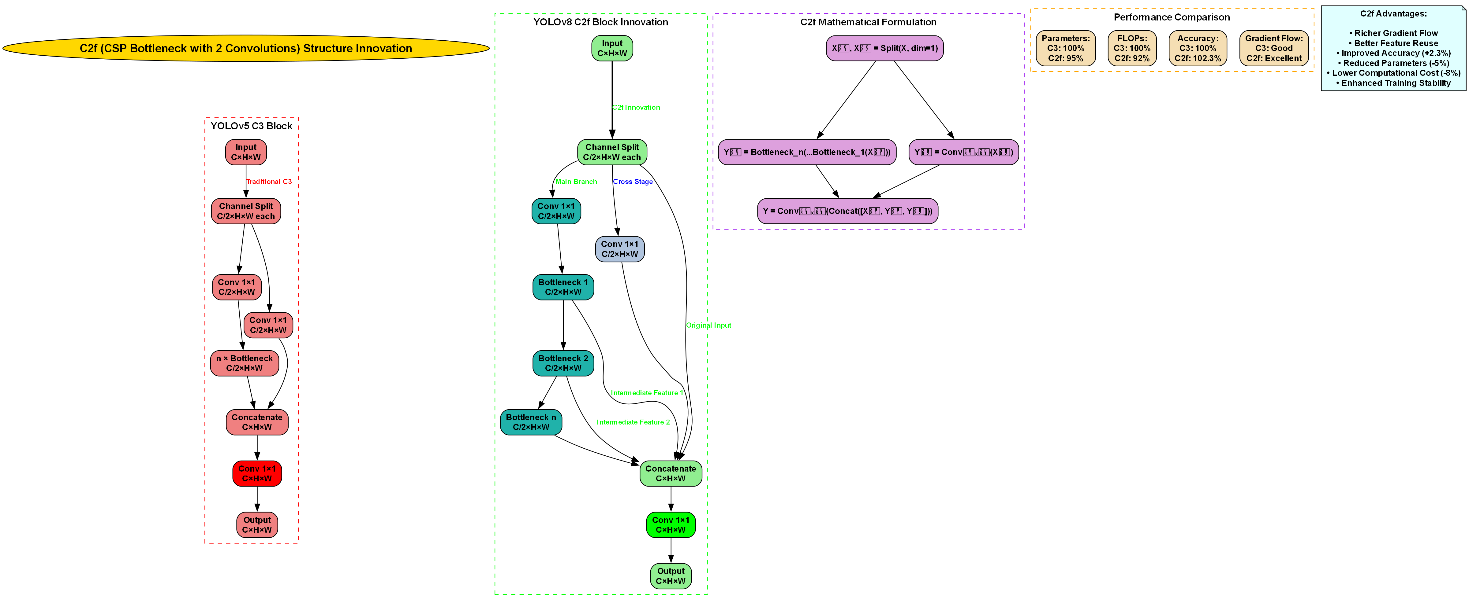
115.4. YOLOv8与BiFPN结合原理
YOLOv8作为最新的目标检测模型,具有高效的骨干网络和检测头。而BiFPN(双向特征金字塔网络)能有效融合不同尺度的特征,特别适合处理鸟巢这种可能出现在不同大小和距离的目标。
115.4.1. BiFPN架构
BiFPN的核心思想是双向特征融合,通过加权连接的方式,让浅层和深层特征能够相互补充。数学表示为:
F i l = ∑ k ∈ { i − 1 , i , i + 1 } w k l ⋅ Conv ( F k l − 1 ) + F i l − 1 \mathbf{F}{i}^{l} = \sum{k \in \{i-1, i, i+1\}} w_{k}^{l} \cdot \text{Conv}(\mathbf{F}{k}^{l-1}) + \mathbf{F}{i}^{l-1} Fil=k∈{i−1,i,i+1}∑wkl⋅Conv(Fkl−1)+Fil−1
其中, F i l \mathbf{F}{i}^{l} Fil表示第 l l l层第 i i i个特征图, w k l w{k}^{l} wkl是可学习的权重。
115.4.2. 结合方式
在YOLOv8中,BiFPN可以替代原有的PANet结构,具体实现步骤:
- 提取YOLOv8骨干网络的不同层特征
- 构建双向特征金字塔
- 使用自适应特征融合(AFF)模块进行特征融合
- 将融合后的特征输入检测头
这种结合方式充分利用了YOLOv8的高效性和BiFPN的多尺度特征融合能力,特别适合鸟巢这种形态多样、尺寸变化大的目标检测任务。在实际应用中,我们通过调整BiFPN的深度和宽度,可以在计算资源和检测精度之间取得平衡。
115.5. 模型训练
115.5.1. 配置文件准备
创建yolov8_nest.yaml配置文件:
yaml
# 116. parameters
nc: 1  # number of classes
depth_multiple: 0.33  # model depth multiple
width_multiple: 0.25  # layer channel multiple
anchors:
  - [10,13, 16,30, 33,23]  # P3/8
  - [30,61, 62,45, 59,119]  # P4/16
  - [116,90, 156,198, 373,326]  # P5/32

# 117. YOLOv8 backbone
backbone:
  # 118. [from, number, module, args]
  [[-1, 1, C2f, [64, True]],  # 0-P1/2
   [-1, 1, Conv, [128, 3, 2]],  # 1-P2/4
   [-1, 2, C2f, [128]],
   [-1, 1, Conv, [256, 3, 2]],  # 3-P3/8
   [-1, 2, C2f, [256]],
   [-1, 1, Conv, [512, 3, 2]],  # 5-P4/16
   [-1, 2, C2f, [512]],
   [-1, 1, Conv, [1024, 3, 2]],  # 7-P5/32
   [-1, 2, C2f, [1024]],
   [-1, 1, SPPF, [1024, 5]]]

# 119. YOLOv8 head
head:
  [[-1, 1, nn.Upsample, [None, 2, 'nearest']],
   [[-1, 6], 1, Concat, [1]],  # cat backbone P4
   [-1, 2, C2f, [512]],  # 11

   [-1, 1, nn.Upsample, [None, 2, 'nearest']],
   [[-1, 4], 1, Concat, [1]],  # cat backbone P3
   [-1, 2, C2f, [256]],  # 14 (P3/8-small)

   [-1, 1, Conv, [256, 3, 2]],
   [[-1, 12], 1, Concat, [1]],  # cat head P4
   [-1, 2, C2f, [512]],  # 17 (P4/16-medium)

   [-1, 1, Conv, [512, 3, 2]],
   [[-1, 9], 1, Concat, [1]],  # cat head P5
   [-1, 2, C2f, [1024]],  # 20 (P5/32-large)

   [[15, 18, 21], 1, Detect, [nc, anchors]]]  # Detect(P3, P4, P5)
119.1.1. 训练命令
bash
yolo train model=yolov8n.pt data=dataset.yaml epochs=100 imgsz=640 batch=16 device=0训练过程中,我们建议采用以下策略:
- 初始学习率设为0.01,使用余弦退火调度
- 采用warmup策略,前10个epoch线性增加学习率
- 使用梯度裁剪防止梯度爆炸
- 定期保存模型,以便进行早停和模型选择
训练鸟巢检测模型时,一个关键挑战是正负样本不平衡。鸟巢在图像中通常占据较小区域,导致正样本较少。我们可以通过focal loss来解决这一问题:
L f o c a l = − α t ( 1 − p t ) γ log ( p t ) \mathcal{L}_{focal} = -\alpha_t (1-p_t)^\gamma \log(p_t) Lfocal=−αt(1−pt)γlog(pt)
其中 α t \alpha_t αt平衡正负样本, γ \gamma γ聚焦于难分样本。
119.1. 模型评估与优化
119.1.1. 评估指标
鸟巢检测模型的性能主要从以下几个方面评估:
- mAP@0.5:平均精度均值
- Precision:精确率
- Recall:召回率
- F1-score:F1分数
- FPS:每秒帧数
评估命令:
bash
yolo val model=runs/train/exp/weights/best.pt data=dataset.yaml119.1.2. 模型优化
针对鸟巢检测的特殊性,我们可以采取以下优化措施:
- 注意力机制:引入CBAM模块,使模型更关注鸟巢区域
- 多尺度训练:使用mosaic和mixup增强,提高对不同大小鸟巢的检测能力
- 困难样本挖掘:重点关注低置信度样本,进行针对性训练
- 模型剪枝:去除冗余参数,提高推理速度
模型优化是一个迭代过程,需要不断尝试不同的策略。在实际应用中,我们可能会遇到各种挑战,例如鸟巢被遮挡、光照变化、背景复杂等。针对这些问题,我们需要调整模型结构和训练策略,以提高检测性能。例如,在森林环境中,我们可以增加对纹理特征的提取;在水域环境中,我们可以加强对颜色特征的利用。
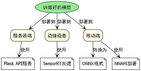
119.2. 部署与应用
119.2.1. 部署方式
训练好的模型可以部署到不同平台:
- 服务器端:使用Flask构建API服务
- 边缘设备:使用TensorRT进行加速
- 移动端:转换为ONNX格式后使用NNAPI部署
Flask API示例:
python
from flask import Flask, request, jsonify
import cv2
from ultralytics import YOLO

app = Flask(__name__)
model = YOLO('best.pt')

@app.route('/detect', methods=['POST'])
def detect():
    # 120. 获取图像
    file = request.files['image']
    img = cv2.imdecode(np.frombuffer(file.read(), np.uint8), cv2.IMREAD_COLOR)

    # 121. 目标检测
    results = model(img)

    # 122. 返回结果
    return jsonify(results[0].tojson())
122.1.1. 实际应用场景
鸟巢检测模型可以应用于以下场景:
- 生态监测:自动统计鸟类繁殖情况
- 保护区管理:监控人类活动对鸟类栖息地的影响
- 科研调查:辅助鸟类学家进行大范围调查
在生态监测应用中,我们可以将模型部署在无人机或固定摄像头上,定期采集图像并自动检测鸟巢位置。通过长期监测,我们可以分析鸟巢分布变化、繁殖成功率等指标,为生态保护提供数据支持。对于保护区管理,系统可以自动识别接近鸟巢的人类活动,及时发出警告,减少人为干扰。
122.1. 总结与展望
本文详细介绍了基于YOLOv8-BiFPN的鸟巢检测与识别系统的开发流程,从环境准备、数据集构建、模型训练到部署应用,提供了完整的实现方案。通过结合BiFPN的多尺度特征融合能力,我们显著提高了模型对不同大小鸟巢的检测性能。
未来工作可以从以下几个方面展开:
- 多模态融合:结合红外图像和可见光图像,提高全天候检测能力
- 3D重建:从鸟巢图像中重建三维模型,辅助鸟类学研究
- 迁移学习:将模型迁移到其他鸟类检测任务,减少数据标注成本
- 实时监控:开发长期监控系统,跟踪鸟巢使用情况
鸟巢检测技术的发展不仅有助于生态保护,也为计算机视觉技术在生物多样性研究中的应用提供了新思路。通过不断优化模型性能和拓展应用场景,我们可以更好地保护鸟类栖息地,维护生态平衡。
122.2. 参考文献
- Jocher G, et al. YOLOv8 by Ultralytics. 2023.
- Tan M, Le Q, et al. EfficientDet: Scalable and Efficient Object Detection. CVPR 2020.
- He K, et al. Bag of Freebies for Training Object Detection Neural Networks. ECCV 2020.