神经网络激活函数完整指南
1. 什么是激活函数
激活函数(Activation Function)是神经网络中的核心组件,它决定了神经元是否应该被"激活"。没有激活函数,神经网络只能学习线性关系,即使堆叠多层也等价于单层线性变换。
1.1 激活函数的作用
| 作用 | 说明 |
|---|---|
| 引入非线性 | 使网络能够学习复杂的非线性模式 |
| 控制输出范围 | 将神经元输出限制在特定范围内 |
| 梯度流动 | 决定反向传播时梯度的传播方式 |
| 特征映射 | 帮助网络学习不同层次的特征表示 |
1.2 数学定义
激活函数本质是一个非线性函数 f(x):
y=f(z)=f(∑wixi+b)y = f(z) = f(\sum w_i x_i + b)y=f(z)=f(∑wixi+b)
其中:
x_i- 输入信号w_i- 权重参数b- 偏置项z- 线性组合结果y- 神经元输出
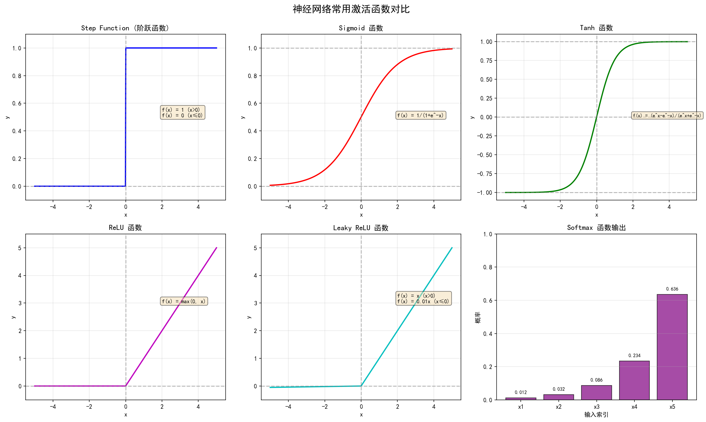
2. 常用激活函数详解
2.1 Step Function(阶跃函数)
最简单的激活函数,模拟生物神经元的"全有或全无"特性。
数学公式:
f(x)={1x>00x≤0f(x) = \begin{cases} 1 & x > 0 \\ 0 & x \leq 0 \end{cases}f(x)={10x>0x≤0
代码实现:
python
import numpy as np
import matplotlib.pyplot as plt

def step_function(x):
    return np.array(x > 0, dtype=int)

x = np.arange(-5.0, 5.0, 0.1)
y = step_function(x)
plt.plot(x, y)
plt.ylim(-0.1, 1.1)
plt.show()
特点:
- ✅ 计算简单
- ✅ 生物可解释性强
- ❌ 导数为0,无法使用梯度下降
- ❌ 无法输出概率值
应用场景: 早期感知机模型,现在很少使用
2.2 Sigmoid 函数
Sigmoid 是最常用的激活函数之一,将输出映射到(0,1)区间。
数学公式:
f(x)=11+e−xf(x) = \frac{1}{1 + e^{-x}}f(x)=1+e−x1
代码实现:
python
def sigmoid(x):
    return 1 / (1 + np.exp(-x))

# 测试
print(sigmoid(0))     # 0.5
print(sigmoid(3.14))  # 约 0.96
特点:
- ✅ 输出在(0,1),可表示概率
- ✅ 导数平滑,便于梯度计算
- ❌ 梯度消失问题:导数最大值为0.25
- ❌ 输出不是零中心
- ❌ 计算成本较高
梯度消失演示:
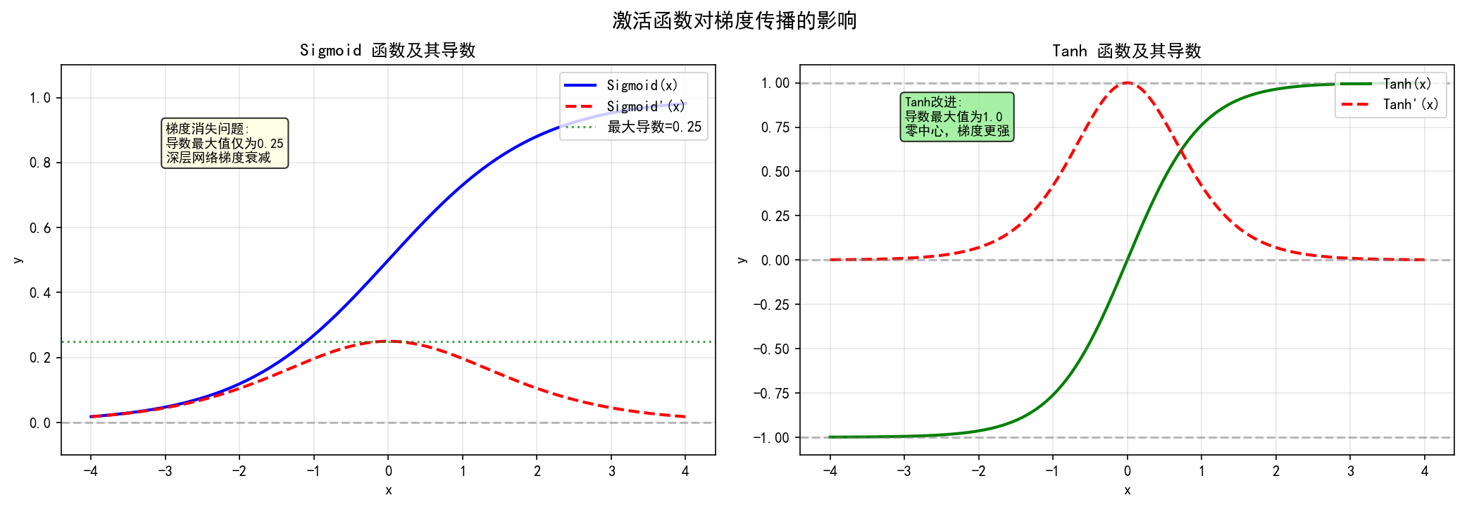
注意:当使用Sigmoid作为激活函数时,深层网络的梯度会逐层衰减,导致靠近输入层的权重几乎无法更新。
2.3 Tanh 函数
双曲正切函数,是Sigmoid的零中心版本。
数学公式:
f(x)=ex−e−xex+e−xf(x) = \frac{e^x - e^{-x}}{e^x + e^{-x}}f(x)=ex+e−xex−e−x
代码实现:
python
def tanh(x):
    return (np.exp(x) - np.exp(-x)) / (np.exp(x) + np.exp(-x))
# 或直接使用 numpy
# y = np.tanh(x)
特点:
- ✅ 输出在(-1,1),零中心
- ✅ 导数最大值为1,梯度更强
- ❌ 仍然存在梯度消失问题
- ❌ 计算成本较高
与Sigmoid对比:
- Tanh的梯度比Sigmoid更"陡峭"
- 零中心特性使梯度传播更均匀
2.4 ReLU 函数
Rectified Linear Unit(修正线性单元),目前最常用的隐藏层激活函数。
数学公式:
f(x)=max(0,x)={xx>00x≤0f(x) = \max(0, x) = \begin{cases} x & x > 0 \\ 0 & x \leq 0 \end{cases}f(x)=max(0,x)={x0x>0x≤0
代码实现:
python
def relu(x):
    return np.maximum(0, x)
特点:
- ✅ 计算极其简单(只需比较操作)
- ✅ 梯度不会饱和(正区间)
- ✅ 收敛速度快(比Sigmoid快6倍)
- ❌ Dying ReLU问题:负区间梯度为0,可能导致神经元"死亡"
Dying ReLU示意:
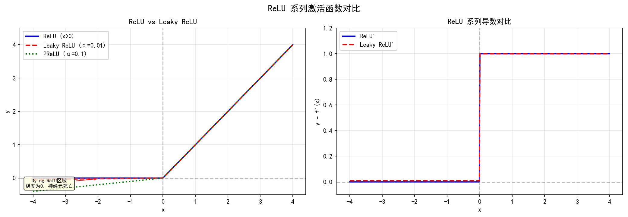
2.5 Leaky ReLU
ReLU的改进版本,解决Dying ReLU问题。
数学公式:
f(x)={xx>0αxx≤0f(x) = \begin{cases} x & x > 0 \\ \alpha x & x \leq 0 \end{cases}f(x)={xαxx>0x≤0
其中 α\alphaα 通常取0.01。
代码实现:
python
def leaky_relu(x, alpha=0.01):
    return np.where(x > 0, x, alpha * x)
特点:
- ✅ 负区间有微小梯度,不会"死亡"
- ✅ 保持ReLU的优点
- ✅ 实践中效果稳定
- ❌ α\alphaα 需要手动调参
2.6 Softmax 函数
Softmax用于多分类问题的输出层,将输出转换为概率分布。
数学公式:
f(xi)=exi∑j=1nexjf(x_i) = \frac{e^{x_i}}{\sum_{j=1}^{n} e^{x_j}}f(xi)=∑j=1nexjexi
代码实现:
python
def softmax(x):
    """计算softmax,防止数值溢出"""
    max_x = np.max(x)  # 减去最大值防止溢出
    exp_x = np.exp(x - max_x)
    return exp_x / np.sum(exp_x)

# 示例
inputs = [0.3, 2.9, 4.0]
print(softmax(inputs))  # 输出概率分布
特点:
- ✅ 输出为概率分布,总和为1
- ✅ 强调最大值,抑制小值
- ❌ 仅用于多分类输出层
- ❌ 需要处理数值溢出
3. 激活函数在神经网络中的应用
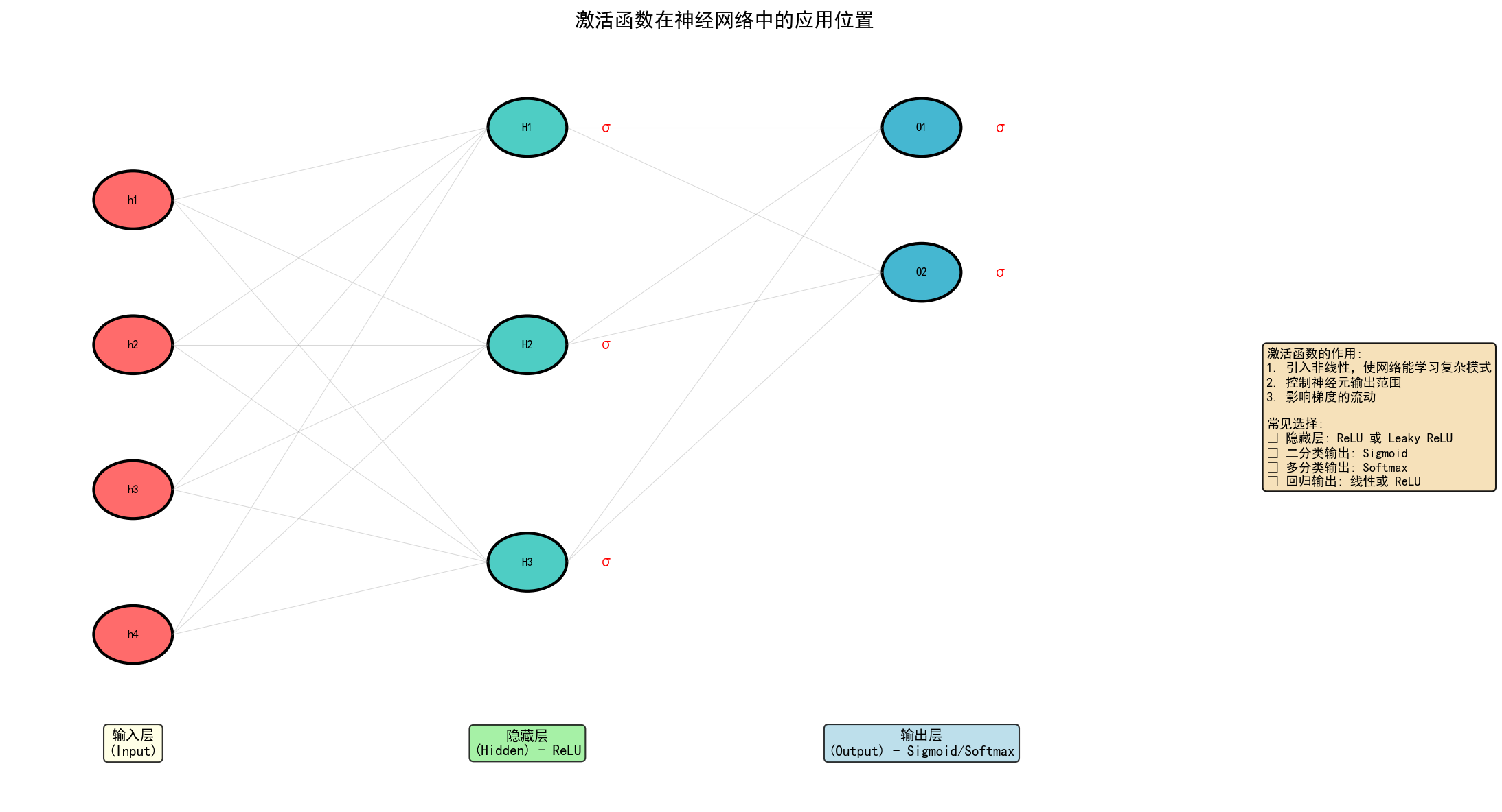
3.1 常见配置
| 网络位置 | 推荐激活函数 | 原因 |
|---|---|---|
| 隐藏层 | ReLU / Leaky ReLU | 梯度流动好,计算高效 |
| 二分类输出 | Sigmoid | 输出(0,1)概率 |
| 多分类输出 | Softmax | 概率分布,总和为1 |
| 回归输出 | Linear / ReLU | 无范围限制 |
3.2 代码示例
python
import numpy as np

class NeuralNetwork:
    def __init__(self, layer_sizes):
        """
        创建一个多层神经网络
        layer_sizes: [输入层, 隐藏层1, 隐藏层2, ..., 输出层]
        """
        self.weights = []
        self.biases = []

        # 初始化权重和偏置
        for i in range(len(layer_sizes) - 1):
            w = np.random.randn(layer_sizes[i], layer_sizes[i+1]) * 0.01
            b = np.zeros((1, layer_sizes[i+1]))
            self.weights.append(w)
            self.biases.append(b)

    def relu(self, x):
        return np.maximum(0, x)

    def sigmoid(self, x):
        return 1 / (1 + np.exp(-np.clip(x, -500, 500)))

    def softmax(self, x):
        exp_x = np.exp(x - np.max(x, axis=1, keepdims=True))
        return exp_x / np.sum(exp_x, axis=1, keepdims=True)

    def forward(self, X):
        """前向传播"""
        self.activations = [X]

        for i in range(len(self.weights) - 1):
            z = np.dot(self.activations[-1], self.weights[i]) + self.biases[i]
            a = self.relu(z)  # 隐藏层用ReLU
            self.activations.append(a)

        # 输出层
        z_out = np.dot(self.activations[-1], self.weights[-1]) + self.biases[-1]
        output = self.softmax(z_out)  # 多分类用Softmax

        return output

# 使用示例
nn = NeuralNetwork([784, 256, 128, 10])  # MNIST网络结构
4. 梯度消失问题详解
4.1 问题本质
在反向传播中,梯度需要逐层传递回输入层:
δ(l)=∂E∂z(l)=δ(l+1)⋅W(l+1)⋅f′(z(l))\delta^{(l)} = \frac{\partial E}{\partial z^{(l)}} = \delta^{(l+1)} \cdot W^{(l+1)} \cdot f'(z^{(l)})δ(l)=∂z(l)∂E=δ(l+1)⋅W(l+1)⋅f′(z(l))
如果激活函数的导数 ∣f′(x)∣<1|f'(x)| < 1∣f′(x)∣<1,则梯度会指数级衰减。
4.2 各函数梯度对比
| 激活函数 | 导数范围 | 深层网络表现 |
|---|---|---|
| Sigmoid | (0, 0.25] | 严重梯度消失 |
| Tanh | (0, 1] | 仍有梯度消失 |
| ReLU | {0, 1} | 无梯度消失 |
4.3 解决方案
- 使用ReLU系列 - 避免正区间饱和
- Batch Normalization - 稳定每层输入分布
- 残差连接(ResNet) - 提供梯度直接通道
- LSTM/GRU - 门控机制控制梯度
5. 激活函数选择指南

5.1 决策流程
1. 网络类型是什么?
   ├── 隐藏层 → 使用 ReLU 或 Leaky ReLU
   └── 输出层 → 根据任务类型选择
               ├── 二分类 → Sigmoid
               ├── 多分类 → Softmax
               └── 回归 → Linear(无激活)

2. 是否遇到Dying ReLU?
   ├── 是 → 改用 Leaky ReLU / PReLU / ELU
   └── 否 → 继续使用 ReLU

3. 是否需要输出概率?
   ├── 是 → Sigmoid 或 Softmax
   └── 否 → ReLU / Tanh / Linear
5.2 实践建议
初学者建议配置:
python
# 推荐配置
hidden_activation = 'relu'      # 隐藏层
output_activation = 'softmax'   # 多分类
# 或
output_activation = 'sigmoid'   # 二分类
调参建议:
- 如果准确率突然下降,检查是否有Dying ReLU
- 尝试Leaky ReLU(α=0.01~0.3)
- Tanh在RNN中效果通常比ReLU好
- 复杂网络可以尝试ELU或SELU
6. 代码演示
6.1 独立函数测试
python
# 独立测试各激活函数

import numpy as np
import matplotlib.pyplot as plt

# 定义激活函数
def step_function(x):
    return np.array(x > 0, dtype=int)

def sigmoid(x):
    return 1 / (1 + np.exp(-x))

def tanh(x):
    return np.tanh(x)

def relu(x):
    return np.maximum(0, x)

def leaky_relu(x, alpha=0.01):
    return np.where(x > 0, x, alpha * x)

def softmax(x):
    exp_x = np.exp(x - np.max(x))
    return exp_x / np.sum(exp_x)

# 测试数据
x = np.linspace(-4, 4, 100)

# 绘制对比图
fig, axes = plt.subplots(2, 3, figsize=(15, 10))

functions = [
    ('Step', step_function),
    ('Sigmoid', sigmoid),
    ('Tanh', tanh),
    ('ReLU', relu),
    ('Leaky ReLU', leaky_relu),
]

for ax, (name, func) in zip(axes.flat[:5], functions):
    y = func(x)
    ax.plot(x, y, 'b-', linewidth=2)
    ax.axhline(0, color='gray', linestyle='--', alpha=0.5)
    ax.axvline(0, color='gray', linestyle='--', alpha=0.5)
    ax.set_title(f'{name}')
    ax.grid(True, alpha=0.3)
    ax.set_ylim(-1.5, 5)

# Softmax示例
inputs = np.array([1.0, 2.0, 3.0, 4.0])
y_softmax = softmax(inputs)
ax6 = axes[1, 2]
ax6.bar(range(len(inputs)), y_softmax, color='purple', alpha=0.7)
ax6.set_title('Softmax Output')
ax6.set_xlabel('Input Index')
ax6.set_ylabel('Probability')

plt.tight_layout()
plt.savefig('activation_functions.png', dpi=150)
plt.show()
6.2 导数计算
python
# 计算各激活函数的导数

def sigmoid_derivative(x):
    s = sigmoid(x)
    return s * (1 - s)

def tanh_derivative(x):
    t = tanh(x)
    return 1 - t**2

def relu_derivative(x):
    return np.where(x > 0, 1, 0)

# 验证导数
x = np.linspace(-4, 4, 100)
print("Sigmoid导数最大值:", max(sigmoid_derivative(x)))
print("Tanh导数最大值:", max(tanh_derivative(x)))
print("ReLU导数范围:", relu_derivative(x).min(), "~", relu_derivative(x).max())